AI Trading Systems That Adapt to Market Conditions

Introduction: The Strategy That Worked Last Year Is Already Obsolete

In 2021, a simple momentum strategy applied to crypto would have made you look like a genius. Buy what was going up; it kept going up. Trend-following systems posted extraordinary returns. Volatility was high but directional. The market rewarded aggression.

In 2022, that same strategy would have destroyed your account. The macro regime shifted — rising interest rates, collapsing liquidity, risk-off sentiment across all asset classes — and momentum signals that had been reliably profitable inverted. Traders who had not adapted lost not just their 2022 gains but much of what they had earned in 2021.

This is the central problem of algorithmic trading that almost no beginner-to-intermediate resource addresses directly: a strategy that is not designed to adapt is not a strategy — it is a bet on regime persistence. And regimes, by definition, end.

The solution is not to build a better static model. It is to build systems that detect when market conditions change and respond accordingly — systems that carry different playbooks for trending markets, ranging markets, high-volatility regimes, and low-volatility environments, and route signals through the appropriate playbook based on current conditions.

In this post, you will learn exactly how to build adaptive AI trading systems. You will understand Hidden Markov Model-based regime detection, online learning that updates model parameters in real time, ensemble architectures that weight different strategies by regime, and the foundations of reinforcement learning for trading. Code is included throughout. By the end, you will have a clear architectural blueprint for a trading system that is designed to survive — not just in the markets of today, but in the markets of next year.

The Anatomy of a Static System's Failure

Before building adaptive systems, it is worth being precise about why static systems fail. The failure mode is elegant in its predictability.

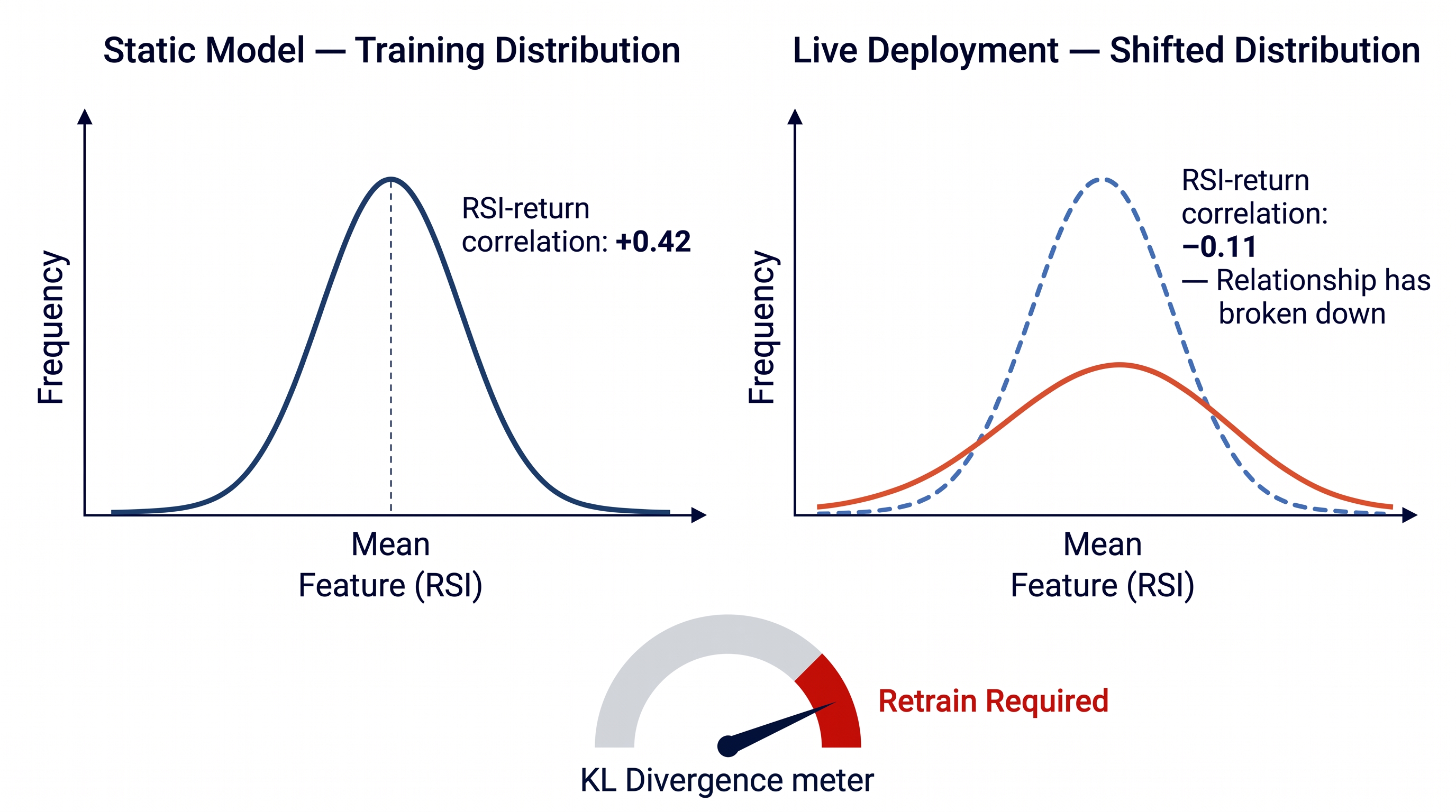
Every machine learning model trained on historical data implicitly assumes that the statistical relationships it learned will persist into the future. A Random Forest trained on 2019–2021 data learns that RSI below 30 combined with high volume tends to precede upward moves. That relationship held in a particular macro environment — one characterized by zero interest rates, institutional FOMO, and retail speculation. When that environment ended, the relationship weakened, then inverted in some regimes entirely.

The formal description of this problem is distribution shift — the training distribution diverges from the deployment distribution . A static model has no mechanism for detecting or responding to this divergence.

The Kullback-Leibler divergence measures the distance between two distributions:

When between your training distribution and the current market distribution exceeds a meaningful threshold, your model's predictions are based on relationships that no longer hold. An adaptive system monitors this divergence and triggers retraining or regime switching when it exceeds a threshold.

Regime Detection: Teaching Your System to Read the Market

The first layer of any adaptive trading system is regime detection — a model or rule set that classifies the current market state into one of several distinct regimes, each associated with different expected asset behavior.

Four regimes cover the majority of market environments: trending up, trending down, ranging (low directional conviction), and high-volatility crisis. Each regime has a distinct signal-generating strategy that performs best within it.

Rule-Based Regime Detection

The simplest regime detection approach uses observable market indicators — ADX for trend strength, realized volatility for regime type, and EMA slope for direction:

1import pandas as pd
2import numpy as np
3
4def detect_regime_rules(df, adx_threshold=25, vol_lookback=20,
5ema_period=200, vol_multiplier=1.5):

"""

Rule-based market regime detection using ADX, volatility, and EMA slope.

Returns regime labels: 'uptrend', 'downtrend', 'ranging', 'crisis'

"""

1close = df['close']
2
3# 200-period EMA and slope
4ema200 = close.ewm(span=ema_period, adjust=False).mean()
5ema_slope = ema200.diff(5) / ema200.shift(5)
6
7# Realized volatility (20-period annualized)
8log_ret = np.log(close / close.shift(1))
9vol = log_ret.rolling(vol_lookback).std() * np.sqrt(365)
10vol_long = log_ret.rolling(vol_lookback * 3).std() * np.sqrt(365)
11
12# Use ADX already computed in df or compute basic proxy
13# For this example, use volatility ratio as trend strength proxy
14vol_ratio = vol / vol_long

regimes = []

for i in range(len(df)):

1current_vol_ratio = vol_ratio.iloc[i] if i < len(vol_ratio) else np.nan
2current_slope = ema_slope.iloc[i] if i < len(ema_slope) else np.nan
3current_vol = vol.iloc[i] if i < len(vol) else np.nan
4long_vol = vol_long.iloc[i] if i < len(vol_long) else np.nan
5
6if pd.isna(current_vol_ratio) or pd.isna(current_slope):

regimes.append('unknown')

elif current_vol > long_vol * vol_multiplier:

regimes.append('crisis')

elif current_vol_ratio > 1.2 and current_slope > 0:

regimes.append('uptrend')

elif current_vol_ratio > 1.2 and current_slope < 0:

regimes.append('downtrend')

else:

regimes.append('ranging')

1df['regime'] = regimes
2return df

This rule-based approach is interpretable and computationally lightweight. Its limitation is that the thresholds are fixed — they were chosen based on historical observation and may not be optimal as market dynamics evolve. This is where statistical regime detection models offer an advantage.

Hidden Markov Models for Statistical Regime Detection

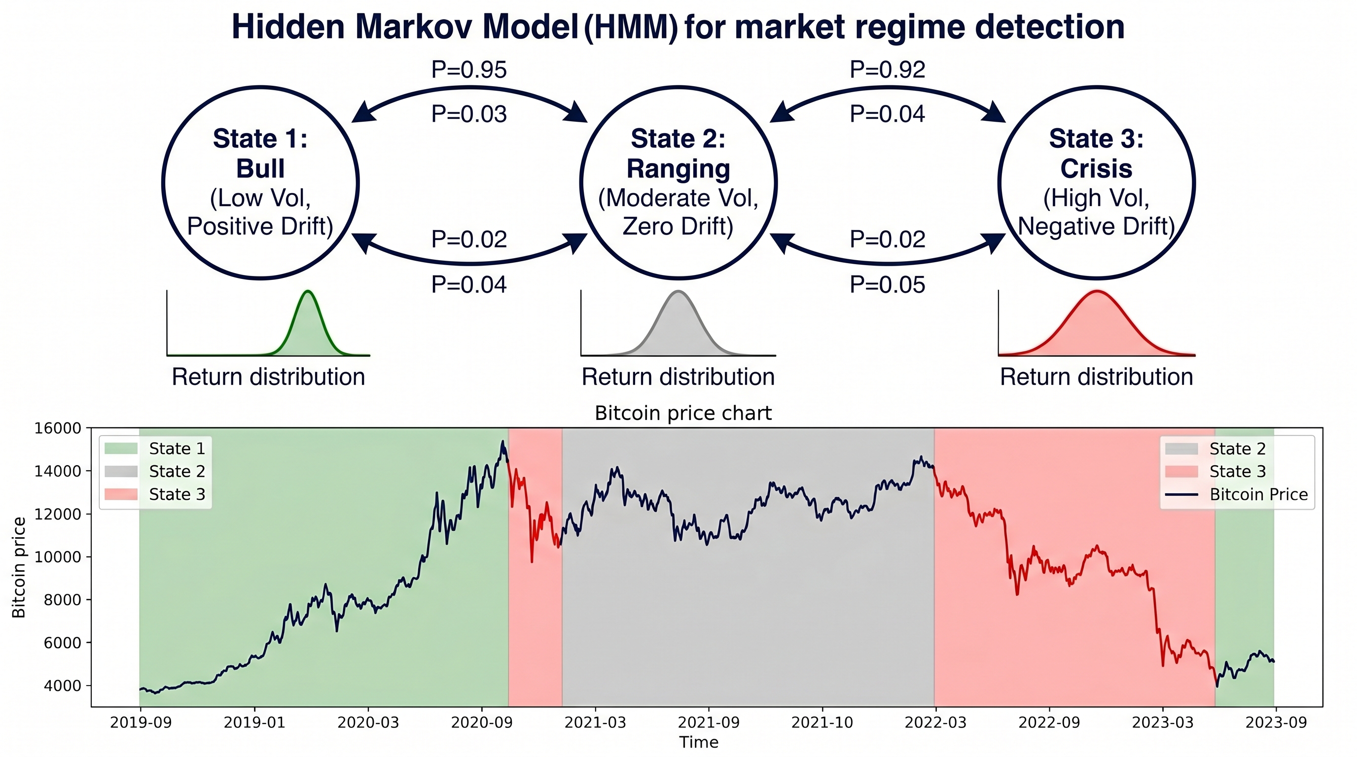
A Hidden Markov Model (HMM) assumes that the market is always in one of hidden states, each generating observable returns with state-specific statistical properties. The model learns the state properties and transition probabilities from data, then infers the current hidden state from the sequence of observed returns.

The likelihood of observing return given that the market is in state follows a Gaussian distribution:

Where and are the mean return and volatility of state . The model also learns a transition matrix where:

This encodes the probability of transitioning from regime to regime . A well-calibrated HMM will learn that high-volatility crisis regimes tend to persist (high self-transition probability) and that transitions from bull to bear states typically pass through a ranging phase.

1from hmmlearn import hmm
2import numpy as np
3import pandas as pd
4
5def fit_hmm_regime_model(returns, n_states=3):

"""

Fit a Gaussian HMM to return series and detect market regimes.

n_states: number of hidden market regimes to identify

"""

1# Prepare observations — reshape for hmmlearn
2obs = returns.dropna().values.reshape(-1, 1)
3
4# Fit Gaussian HMM
5model = hmm.GaussianHMM(
6n_components=n_states,

covariance_type='full',

n_iter=1000,

random_state=42

)

model.fit(obs)

1# Predict hidden states
2hidden_states = model.predict(obs)
3
4# Identify regime characteristics
5state_stats = {}

for state in range(n_states):

mask = hidden_states == state

state_returns = obs[mask]

state_stats[state] = {

1'mean_return': np.mean(state_returns),
2'volatility': np.std(state_returns),
3'frequency': np.mean(mask)
4}
5print(f"State {state}: Mean={np.mean(state_returns):.5f}, "
6f"Vol={np.std(state_returns):.5f}, "
7f"Freq={np.mean(mask):.3f}")
8
9return model, hidden_states, state_stats
10
11# Usage:
12# log_returns = np.log(df['close'] / df['close'].shift(1)).dropna()
13# hmm_model, states, stats = fit_hmm_regime_model(log_returns, n_states=3)

The three states a Gaussian HMM typically discovers in crypto data correspond to: a low-volatility, positive-drift bull state; a moderate-volatility, near-zero-drift ranging state; and a high-volatility, negative-drift crisis state. These states are not labeled by the model — you infer their meaning from the learned mean and variance parameters.

Regime-Conditional Strategy Routing: The Signal Switching Architecture

Detecting the current regime is only half the problem. The other half is routing the right trading strategy through the right regime. This is the signal switching architecture — a meta-layer that sits above your individual strategy models and determines which model's signal is acted upon based on the current detected regime.

1class RegimeConditionalTrader:

"""

Adaptive trading system that routes signals through

regime-specific strategy models.

"""

1def __init__(self):

self.regime_models = {}

self.current_regime = None

1def register_strategy(self, regime_name, model, signal_generator):

"""Register a strategy model for a specific regime."""

self.regime_models[regime_name] = {

'model': model,

'signal_fn': signal_generator

}

1def detect_regime(self, features, hmm_model):

"""Detect current market regime using HMM."""

obs = features['log_return'].values[-20:].reshape(-1, 1)

state = hmm_model.predict(obs)[-1]

1# Map state index to regime name based on learned characteristics
2state_to_regime = {0: 'bull', 1: 'ranging', 2: 'crisis'}

self.current_regime = state_to_regime.get(state, 'ranging')

1return self.current_regime
2
3def generate_signal(self, features):

"""Generate trading signal for the current regime."""

if self.current_regime not in self.regime_models:

1return 0  # No signal if regime has no registered strategy
2
3strategy = self.regime_models[self.current_regime]
4signal = strategy['signal_fn'](features, strategy['model'])
5return signal
6
7def run(self, features_df, hmm_model):

"""Run the adaptive system across a feature DataFrame."""

signals = []

regimes = []

for i in range(20, len(features_df)):

window = features_df.iloc[i-20:i]

regime = self.detect_regime(window, hmm_model)

signal = self.generate_signal(window)

signals.append(signal)

regimes.append(regime)

1return pd.Series(signals), pd.Series(regimes)

Each regime-specific strategy model is trained exclusively on data labeled as that regime — so the bull market model has never seen bear market data and has not learned spurious patterns from the wrong environment. The meta-layer handles the routing; the individual models focus on learning the deepest possible signal within their assigned regime.

Online Learning: Real-Time Model Adaptation

Regime switching handles discrete, detectable shifts in market structure. But markets also drift continuously — subtle, gradual changes in parameter values within a regime that cause a statically trained model to degrade slowly over time. Online learning — the practice of updating model parameters continuously as new data arrives — addresses this.

The most principled approach to online learning uses exponentially weighted updates, giving more recent observations higher weight in parameter estimation:

Where * is the updated parameter estimate, ** is the learning rate, and ** is the gradient of the loss function evaluated on the new observation *. Smaller values weight history more heavily — producing more stable but slower-adapting estimates. Larger values adapt faster but produce noisier estimates.

from sklearn.linear_model import SGDClassifier

1import numpy as np
2
3class OnlineLearningTrader:

"""

Trading model that updates incrementally as new data arrives,

using stochastic gradient descent for real-time adaptation.

"""

1def __init__(self, learning_rate=0.01, regularization=0.001):

self.model = SGDClassifier(

1loss='log_loss',          # Logistic regression loss — gives probabilities

learning_rate='constant',

eta0=learning_rate,

1alpha=regularization,     # L2 regularization
2warm_start=True,          # Preserve weights between partial_fit calls
3random_state=42
4)

self.is_initialized = False

1self.classes = np.array([-1, 0, 1])

self.prediction_history = []

self.update_count = 0

1def initialize(self, X_seed, y_seed):

"""Seed the model with initial training data."""

self.model.partial_fit(X_seed, y_seed, classes=self.classes)

self.is_initialized = True

1print(f"Model initialized on {len(X_seed)} seed observations.")
2
3def predict(self, X):

"""Generate signal with confidence."""

if not self.is_initialized:

1return 0, 0.333
2
3proba = self.model.predict_proba(X.reshape(1, -1))[0]
4class_idx = np.argmax(proba)
5predicted_class = self.classes[class_idx]
6confidence = proba[class_idx]
7
8return predicted_class, confidence
9
10def update(self, X, y_true):

"""Update model with new observation."""

self.model.partial_fit(X.reshape(1, -1), [y_true])

self.update_count += 1

if self.update_count % 100 == 0:

1print(f"Model updated {self.update_count} times.")

The partial_fit method of scikit-learn's SGDClassifier enables true online learning — the model parameters are updated incrementally without retraining from scratch. This is computationally efficient and naturally implements the exponentially decaying weight of older observations that is implicit in gradient descent dynamics.

The tension in online learning is between stability and plasticity. A model that adapts too quickly forgets patterns that are still valid; a model that adapts too slowly fails to capture regime changes. The optimal learning rate is regime-dependent — higher during transition periods, lower during stable regimes. This can be implemented by coupling the online learning rate to the detected regime volatility.

Reinforcement Learning: The Self-Improving Trader

Regime detection and online learning are adaptations to a known framework. Reinforcement learning (RL) takes a fundamentally different approach: it treats trading as a sequential decision problem and learns the optimal policy by interacting with the market environment and receiving reward feedback.

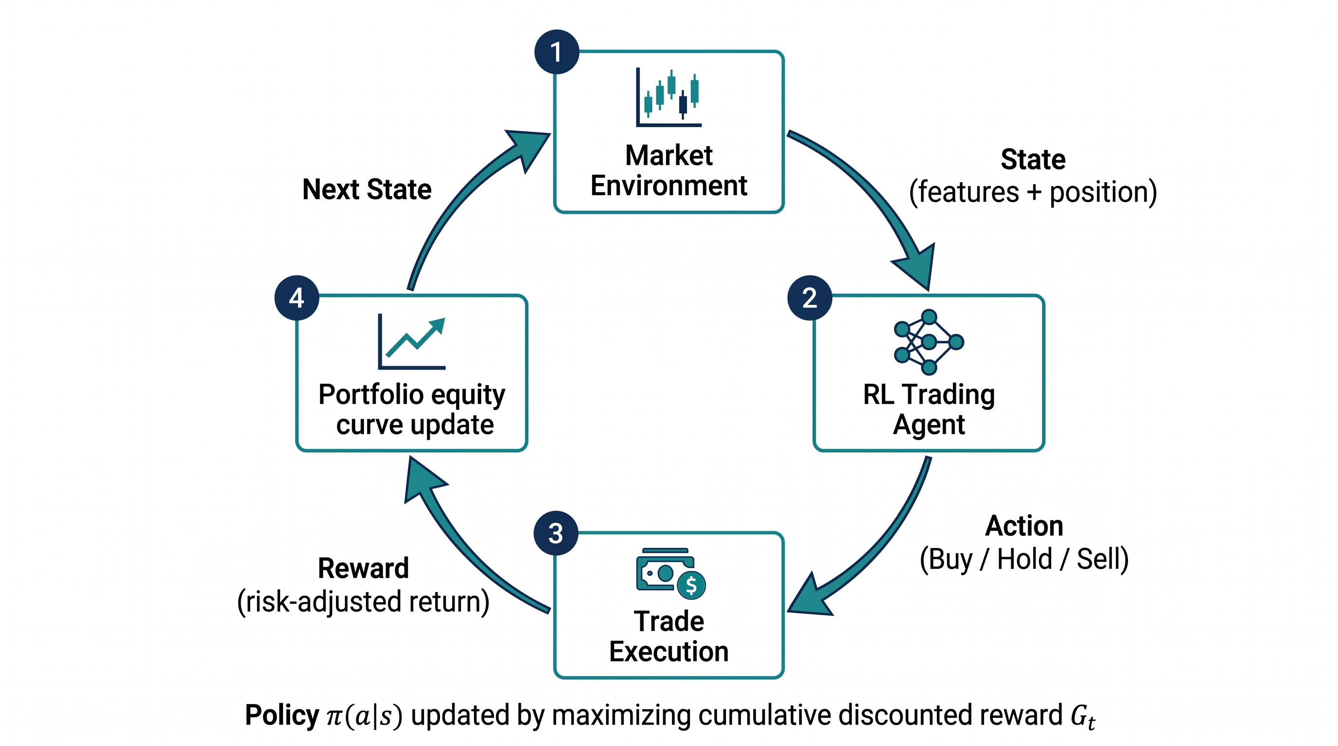
An RL trading agent is defined by four components. The state is the agent's observation of the market — typically a vector of price-derived features and current portfolio position. The action is the trading decision — buy, sell, or hold. The reward is the feedback signal — typically the portfolio return generated by the action. The policy maps states to action probabilities and is what the agent learns to optimize.

The agent's objective is to maximize cumulative discounted reward:

Where is the discount factor — controlling how much the agent weighs immediate versus future rewards. A discount factor close to 1 means the agent plans for long-term outcomes; close to 0 means it optimizes myopically.

1import numpy as np
2
3class TradingEnvironment:

"""

A simple reinforcement learning environment for crypto trading.

Implements the OpenAI Gym interface pattern.

"""

1def __init__(self, price_series, features_df, initial_capital=10000,
2transaction_cost=0.001, window=20):

self.prices = price_series.values

self.features = features_df.values

self.capital = initial_capital

self.initial_capital = initial_capital

self.tc = transaction_cost

self.window = window

self.reset()

1def reset(self):

self.t = self.window

self.position = 0 # -1 short, 0 flat, 1 long

self.capital = self.initial_capital

self.portfolio_value = self.initial_capital

self.done = False

1return self._get_state()
2
3def _get_state(self):

"""Return current state: market features + position."""

market_state = self.features[self.t - self.window:self.t].flatten()

1position_state = np.array([self.position])
2return np.concatenate([market_state, position_state])
3
4def step(self, action):

"""

Execute action and return next state, reward, done flag.

Actions: 0=Sell/Short, 1=Hold, 2=Buy/Long

"""

1# Map action to position
2new_position = action - 1  # {0,1,2} → {-1,0,1}
3
4# Compute return for this step

price_return = (self.prices[self.t] - self.prices[self.t - 1]) / \

self.prices[self.t - 1]

1# Portfolio return
2position_return = self.position * price_return
3
4# Apply transaction cost if position changed

if new_position != self.position:

position_return -= self.tc

1# Update portfolio

self.portfolio_value *= (1 + position_return)

self.position = new_position

1# Reward: portfolio return (risk-adjusted)
2reward = position_return
3
4# Advance time

self.t += 1

self.done = self.t >= len(self.prices) - 1

next_state = self._get_state() if not self.done else None

1return next_state, reward, self.done
2
3def sharpe_ratio(self, returns):

"""Compute annualized Sharpe ratio of episode returns."""

1if np.std(returns) == 0:
2return 0
3return (np.mean(returns) / np.std(returns)) * np.sqrt(252)

The reward function design is the most critical decision in building an RL trading agent. Raw portfolio return is a natural reward, but it does not penalize excessive risk-taking. A risk-adjusted reward that incorporates volatility — essentially a step-level Sharpe contribution — produces agents that learn to balance return against drawdown:

Where is the risk-free rate and is a rolling estimate of return volatility. This reward signal teaches the agent that a 2% return with low volatility is more valuable than a 2% return with high volatility — a preference that aligns with sustainable trading.

The Adaptive Ensemble: Combining Multiple Strategies by Regime Weight

The most robust adaptive systems do not switch entirely between strategies — they blend them, weighting each strategy's signal by its estimated quality in the current market regime. This ensemble approach preserves signal from multiple strategies while concentrating weight on the most regime-appropriate ones.

The blended signal is:

Where is the signal from strategy at time , and is the current weight assigned to that strategy. Weights are normalized so that .

The weight update mechanism uses an exponentially weighted average of each strategy's recent performance:

Where is the rolling Sharpe ratio of strategy over the past periods, and is a temperature parameter controlling how aggressively weight is concentrated on the best-performing strategy. High produces near-winner-take-all weighting; low distributes weight more evenly.

1import numpy as np
2import pandas as pd
3
4class AdaptiveEnsemble:

"""

Ensemble that dynamically weights strategy signals based on

their recent Sharpe ratio performance.

"""

1def __init__(self, strategy_names, lookback=60, temperature=2.0):

self.strategy_names = strategy_names

self.lookback = lookback

self.temperature = temperature

self.return_histories = {name: [] for name in strategy_names}

1def update_returns(self, strategy_returns_dict):

"""Record realized returns for each strategy."""

for name, ret in strategy_returns_dict.items():

if name in self.return_histories:

self.return_histories[name].append(ret)

1def compute_weights(self):

"""Compute softmax weights based on rolling Sharpe ratios."""

1sharpe_estimates = {}

for name in self.strategy_names:

hist = self.return_histories[name][-self.lookback:]

if len(hist) < 10:

sharpe_estimates[name] = 0.0

else:

1mean_ret = np.mean(hist)
2std_ret = np.std(hist)

sharpe_estimates[name] = mean_ret / std_ret if std_ret > 0 else 0.0

1# Softmax weighting
2sharpe_array = np.array(list(sharpe_estimates.values()))
3exp_sharpe = np.exp(self.temperature * sharpe_array)
4weights = exp_sharpe / exp_sharpe.sum()
5
6return dict(zip(self.strategy_names, weights))
7
8def blend_signals(self, signals_dict):

"""Blend strategy signals using current weights."""

weights = self.compute_weights()

blended = sum(weights[name] * signal

for name, signal in signals_dict.items())

1return blended, weights

This ensemble architecture has a self-correcting property: as a strategy degrades in the current regime, its rolling Sharpe falls, its weight decreases, and the system naturally de-emphasizes its signal. When market conditions shift to favor that strategy again, its performance improves, and its weight recovers. No human intervention is required.

Performance Monitoring and Automatic Retraining

An adaptive system without a monitoring layer is incomplete. You need a systematic way to detect when model performance has degraded beyond an acceptable threshold and trigger retraining before losses accumulate.

The Page-Cusum test is a sequential statistical test designed to detect structural breaks — points where the statistical properties of a time series change abruptly:

Where is the cumulative sum at time , is the model's realized return at time , is the expected return under normal operation, and is a slack parameter that controls sensitivity. When exceeds a threshold , a structural break is flagged and retraining is triggered.

1def cusum_monitor(returns, mu_0=0.0001, k=0.0002, h=0.005):

"""

CUSUM test for detecting performance degradation.

Triggers alert when cumulative deviation exceeds threshold h.

"""

C = 0.0

alerts = []

for ret in returns:

C = max(0, C + (ret - mu_0) - k)

if C > h:

alerts.append(True)

1C = 0.0  # Reset after alert

else:

alerts.append(False)

1return alerts

A monitoring system that runs this test daily on realized strategy returns, combined with automatic retraining when an alert fires, creates a closed-loop adaptive system that maintains its edge without constant manual oversight.

Key Takeaways

• Static trading models are bets on regime persistence — they fail when market conditions shift, which they inevitably do. Adaptive systems are designed to detect and respond to regime changes rather than being destroyed by them.
• Hidden Markov Models are the most principled statistical approach to regime detection, learning hidden market states and transition probabilities directly from return data.
• Regime-conditional signal routing assigns different strategy models to different market environments, ensuring each model only operates within the conditions it was trained on.
• Online learning via stochastic gradient descent updates model parameters continuously as new data arrives, addressing the gradual drift within regimes that causes static models to decay.
• Reinforcement learning treats trading as a sequential decision problem with explicit reward feedback, enabling agents to discover trading policies that were not pre-specified by the designer.
• Adaptive ensemble weighting using softmax over rolling Sharpe ratios creates a self-correcting system that automatically concentrates signal on the best-performing strategies in current conditions.
• Performance monitoring with CUSUM tests provides a statistical mechanism for detecting degradation and triggering retraining before losses accumulate to unacceptable levels.

Conclusion: Adaptability Is the Only Durable Edge

The markets of 2026 are different from the markets of 2021. The markets of 2028 will be different again. New participants enter, old participants adapt, liquidity conditions shift, macro regimes rotate, and the statistical relationships that powered last year's edge decay as more capital discovers and arbitrages them away.

In this environment, the only genuinely durable edge is architectural: a system designed to detect change, adapt its behavior, and maintain its edge across the full cycle of market regimes — not just the one that happens to prevail when the system is first deployed.

The building blocks of such a system are all accessible to a Python-familiar algorithmic trader today. Hidden Markov Models in the hmmlearn library. Online learning via scikit-learn's partial_fit. Simple RL environments using the patterns shown above, extendable to stable-baselines3 for more sophisticated policy learning. Adaptive ensemble weighting with nothing more than NumPy arithmetic.

The remaining work is integration — assembling these components into a coherent system, validating each layer with rigorous walk-forward testing, and building the monitoring infrastructure that keeps the system honest over time.

Start with regime detection. Apply a three-state Gaussian HMM to two years of daily returns for your primary trading asset. Visualize the detected regimes against the price history and understand what each state corresponds to. Then build one regime-specific strategy for your most clearly defined regime — the high-volatility crisis state, where behavior is most distinctive and most different from the average.

From there, the system grows one component at a time. That is how every serious adaptive trading system is actually built — not in a single session of inspired architecture, but in the patient, deliberate layering of components that each solve a specific failure mode of the static approach.

The market rewards adaptation. Build systems that adapt.