AI Trading System Architecture Explained: How to Build a System That Actually Works End-to-End

Introduction: The Model Is the Easy Part

Most algo traders who get serious about AI-powered trading spend the majority of their time on the model. They obsess over architecture choices — LSTM versus transformer, Random Forest versus XGBoost — they tune hyperparameters for weeks, and they celebrate when validation AUC ticks above 0.57. Then they try to deploy, and the system falls apart within days.

The data feed disconnects silently. The order sizing logic sends a position ten times larger than intended. The model retrains on stale data. The execution layer ignores slippage. The monitoring dashboard shows everything green while the account bleeds.

Here is the counterintuitive insight that professional quant developers learn, usually painfully: the model is the easy part. Any competent Python developer can train a gradient-boosted classifier on OHLCV features in an afternoon. Building the system that keeps that model running reliably — ingesting clean data, generating signals consistently, executing trades safely, monitoring performance honestly, and retraining intelligently — is the genuinely hard work. And it is the work almost nobody teaches.

In this post, you will learn the complete architecture of a production-grade AI trading system, layer by layer. You will understand what belongs in each component, how the components communicate, where systems most commonly fail, and how to implement each layer in Python. Whether you are deploying your first strategy or rebuilding a system that keeps breaking, this architectural blueprint will give you the structural clarity that months of trial and error eventually produces — compressed into a single, practical guide.

If you leave before the end, you will keep building systems that work in notebooks and fail in production. Stay, and you will finish with the mental model of how every component fits together.

The Seven Layers of a Production AI Trading System

A well-architected AI trading system is not a single script — it is a pipeline of distinct, independently maintainable components, each with a clearly defined responsibility. When systems fail, the failure is almost always in one of these layers, or in the interfaces between them.

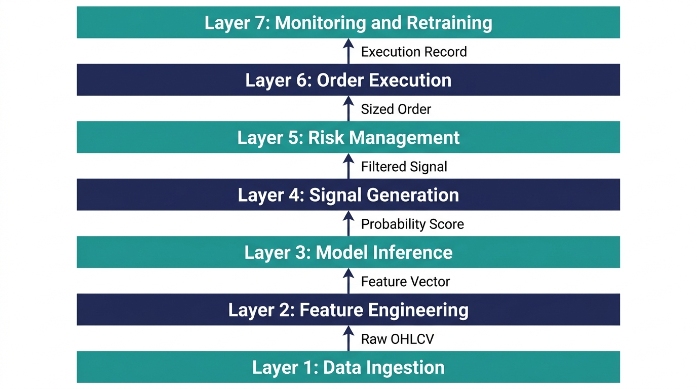
The seven layers are: data ingestion, feature engineering, model inference, signal generation, risk management, order execution, and monitoring and retraining. Each operates independently. Each has defined inputs and outputs. Each can fail independently, and each should be monitored independently.

Layer 1: Data Ingestion — The Foundation That Everything Rests On

If your data pipeline is unreliable, everything built on top of it is unreliable. This layer is responsible for acquiring, validating, storing, and serving market data to the rest of the system — and it needs to do all of this continuously, without silent failures, under real-world network conditions.

Real-Time vs. Historical Data

A production data ingestion layer handles two fundamentally different data modes simultaneously. Historical data — used for model training and backtesting — is typically acquired in batch from exchange APIs or commercial data providers. Real-time data — used for live inference — arrives continuously via WebSocket streams or REST polling, depending on the exchange's API capabilities.

The critical design principle: historical and real-time data must pass through identical normalization and validation logic before any downstream component touches them. This is what makes backtests meaningful — the exact same feature engineering code runs on both historical and live data, ensuring there is no hidden difference between the two modes.

python

1import ccxt
2import pandas as pd
3import time
4import logging
5from datetime import datetime, timezone

logging.basicConfig(level=logging.INFO, format='%(asctime)s — %(levelname)s — %(message)s')

python

1class DataIngestionLayer:

"""

Handles historical OHLCV fetch and basic data validation.

In production, this class is extended with WebSocket streaming

and a persistent database backend (e.g., TimescaleDB or InfluxDB).

"""

python

1def __init__(self, exchange_id='binance', symbol='BTC/USDT', timeframe='1d'):

self.exchange = getattr(ccxt, exchange_id)({'enableRateLimit': True})

self.symbol = symbol

self.timeframe = timeframe

python

1def fetch_ohlcv(self, since_days=365):

"""Fetch historical OHLCV with automatic pagination and validation."""

since_ms = int(

python

1(datetime.now(timezone.utc).timestamp() - since_days * 86400) * 1000
2)

all_candles = []

python

1logging.info(f"Fetching {self.symbol} {self.timeframe} data from {self.exchange.id}")

while True:

candles = self.exchange.fetch_ohlcv(

self.symbol, self.timeframe, since=since_ms, limit=500

)

if not candles:

break

all_candles.extend(candles)

since_ms = candles[-1][0] + 1

python

1time.sleep(self.exchange.rateLimit / 1000)

if len(candles) < 500:

break

python

1df = pd.DataFrame(

all_candles, columns=['timestamp', 'open', 'high', 'low', 'close', 'volume']

)

python

1df['timestamp'] = pd.to_datetime(df['timestamp'], unit='ms', utc=True)
2df.set_index('timestamp', inplace=True)
3
4return self._validate(df)
5
6def _validate(self, df):

"""Data quality validation — fail loudly on bad data rather than silently passing garbage."""

initial_len = len(df)

python

1# Remove duplicate timestamps
2df = df[~df.index.duplicated(keep='last')]
3
4# Remove rows with zero or negative prices
5df = df[(df[['open', 'high', 'low', 'close']] > 0).all(axis=1)]
6
7# Remove rows where high < low (malformed candles)
8df = df[df['high'] >= df['low']]
9
10# Remove rows with zero volume (exchange outages, synthetic fill)
11df = df[df['volume'] > 0]
12
13removed = initial_len - len(df)

if removed > 0:

logging.warning(f"Validation removed {removed} malformed rows ({100*removed/initial_len:.1f}%)")

python

1logging.info(f"Data validated: {len(df)} clean rows, "
2f"{df.index[0].date()} to {df.index[-1].date()}")
3return df.sort_index()

The _validate method is not optional. In production, exchange APIs regularly return malformed candles — zero-volume rows during outages, duplicate timestamps from API glitches, and candles where high is less than low due to data provider errors. Downstream feature engineering components that receive malformed data will produce NaN or infinite feature values that propagate silently through the system and corrupt model inference.

Layer 2: Feature Engineering — Where Raw Data Becomes Predictive Information

Feature engineering is the translation layer between raw market data and the numerical inputs your model can learn from. In a well-architected system, all feature computation lives in a single, version-controlled module that is called identically in training, backtesting, and live inference.

The most common architectural mistake at this layer is having separate feature computation code for training and for live inference. This guarantees that the model eventually receives features computed differently than it was trained on — a silent error that degrades performance gradually and invisibly.

python

1import numpy as np
2import pandas as pd
3
4class FeatureEngineeringLayer:

"""

Computes all model features from validated OHLCV data.

This exact class is used in training, backtesting, and live inference.

Single source of truth for all feature definitions.

"""

python

1def compute_features(self, df: pd.DataFrame) -> pd.DataFrame:
2features = df.copy()
3
4# Log returns
5features['log_return'] = np.log(features['close'] / features['close'].shift(1))
6
7# RSI (14-period)
8delta = features['close'].diff()
9gain = delta.clip(lower=0).rolling(14).mean()
10loss = -delta.clip(upper=0).rolling(14).mean()

features['rsi'] = 100 - (100 / (1 + gain / loss))

python

1# Bollinger Band width
2sma20 = features['close'].rolling(20).mean()
3std20 = features['close'].rolling(20).std()

features['bb_width'] = (2 * std20) / sma20

python

1# Rolling annualized volatility
2features['volatility'] = features['log_return'].rolling(10).std() * np.sqrt(252)
3
4# Volume Z-score
5vol_mean = features['volume'].rolling(20).mean()
6vol_std = features['volume'].rolling(20).std()

features['vol_zscore'] = (features['volume'] - vol_mean) / vol_std

python

1# Lagged returns

for lag in [1, 2, 3, 5, 10]:

python

1features[f'lag_{lag}'] = features['log_return'].shift(lag)
2
3# Drop rows with NaN features (burn-in period from rolling calculations)
4features.dropna(inplace=True)
5
6return features
7
8def get_feature_columns(self):
9return ['rsi', 'bb_width', 'volatility', 'vol_zscore',

'lag_1', 'lag_2', 'lag_3', 'lag_5', 'lag_10']

The Bollinger Band width, expressed as a normalized volatility measure, is computed as:

And annualized rolling volatility as:

Both formulas use only past data at each time step — no centered windows, no future-referencing calculations. This is enforced by the architecture, not left to individual developer discipline.

Layer 3: Model Inference — Turning Features Into Probabilities

The model inference layer receives a feature vector and returns a probability estimate. In a clean architecture, this layer knows nothing about data sources, trading logic, or execution — it simply wraps a trained model and exposes a predict interface.

This separation allows you to swap model architectures — from Random Forest to XGBoost to a neural network — without touching any other system component.

python

1import joblib
2import numpy as np

from sklearn.preprocessing import StandardScaler

from sklearn.ensemble import RandomForestClassifier

python

1class ModelInferenceLayer:

"""

Wraps a trained model and scaler for live inference.

Handles feature scaling, prediction, and confidence scoring.

"""

python

1def __init__(self, model_path='model.joblib', scaler_path='scaler.joblib'):

self.model = joblib.load(model_path)

self.scaler = joblib.load(scaler_path)

python

1self.feature_columns = None  # Set during training, loaded from model metadata
2
3def predict(self, feature_vector: np.ndarray) -> dict:

"""

Returns prediction probability and metadata.

Always returns a structured dict — never a raw float.

"""

scaled = self.scaler.transform(feature_vector.reshape(1, -1))

prob_up = self.model.predict_proba(scaled)[0, 1]

python

1return {
2'probability_up': round(float(prob_up), 4),
3'probability_down': round(float(1 - prob_up), 4),
4'confidence': round(float(abs(prob_up - 0.5) * 2), 4),  # 0 to 1 scale
5'raw_prediction': int(prob_up > 0.5)
6}

@classmethod

python

1def train_and_save(cls, X_train, y_train, feature_cols,

model_path='model.joblib', scaler_path='scaler.joblib'):

"""Train, scale, and persist model and scaler together."""

scaler = StandardScaler()

X_scaled = scaler.fit_transform(X_train)

model = RandomForestClassifier(

n_estimators=300, max_depth=6, min_samples_leaf=20,

class_weight='balanced', random_state=42, n_jobs=-1

)

model.fit(X_scaled, y_train)

joblib.dump(model, model_path)

joblib.dump(scaler, scaler_path)

python

1print(f"Model and scaler saved to {model_path}, {scaler_path}")
2return cls(model_path, scaler_path)

The confidence field deserves explanation. Raw probability outputs from classification models range from 0 to 1, where 0.5 represents maximum uncertainty. The confidence score transforms this into a 0-to-1 scale where 0 means the model is completely uncertain and 1 means the model is completely certain in either direction:

This makes downstream signal filtering intuitive — trade only when confidence exceeds a threshold, regardless of direction.

Layer 4: Signal Generation — From Probability to Trading Decision

The signal generation layer applies filtering logic to the raw model output to produce actionable trading decisions. It is responsible for confidence thresholding, signal deduplication, and optionally regime filtering.

python

1from dataclasses import dataclass
2from typing import Optional
3from datetime import datetime

@dataclass

python

1class TradingSignal:

timestamp: datetime

direction: str # 'long', 'short', or 'flat'

confidence: float # 0 to 1

probability_up: float

source_model: str

regime: Optional[str] = None

python

1class SignalGenerationLayer:

"""

Converts model inference output into structured trading signals.

Applies confidence filtering and signal deduplication.

"""

python

1def __init__(self, confidence_threshold=0.30, min_signal_interval_bars=1):

self.confidence_threshold = confidence_threshold

self.min_signal_interval_bars = min_signal_interval_bars

self.last_signal_bar = -999

python

1def generate_signal(self, inference_result: dict,

current_bar: int,

current_time: datetime,

model_name: str = 'primary') -> Optional[TradingSignal]:

"""

Returns a TradingSignal if confidence meets threshold,

None if the model is uncertain or signal is too frequent.

"""

confidence = inference_result['confidence']

prob_up = inference_result['probability_up']

python

1# Confidence filter — only act on strong model convictions

if confidence < self.confidence_threshold:

python

1return None
2
3# Deduplication — prevent redundant signals on consecutive bars

if (current_bar - self.last_signal_bar) < self.min_signal_interval_bars:

python

1return None

direction = 'long' if prob_up > 0.5 else 'short'

self.last_signal_bar = current_bar

python

1return TradingSignal(
2timestamp=current_time,
3direction=direction,
4confidence=confidence,
5probability_up=prob_up,
6source_model=model_name
7)

The confidence threshold of 0.30 on the normalized scale corresponds to a raw probability above approximately 0.65 for long signals. Adjusting this threshold is a critical system parameter — higher thresholds produce fewer but higher-quality signals, lower thresholds produce more signals with lower average quality. The optimal value is strategy and asset specific and should be determined through walk-forward backtesting.

Layer 5: Risk Management — The System That Keeps You in the Game

The risk management layer sits between the signal and the exchange. It receives a trading signal and returns a sized, risk-adjusted order — or no order at all if position limits, drawdown limits, or volatility conditions prevent trading.

This is not optional sophistication. It is the difference between a system that survives adverse periods and one that generates a single catastrophic loss.

Position Sizing with the Kelly Criterion

The Kelly Criterion provides a mathematically optimal position size that maximizes the long-run geometric growth rate of capital, given an edge and a win rate:

Where $f^{*}$ is the fraction of capital to risk, $p$ is the probability of winning (from model output), $q = 1 - p$ is the probability of losing, and $b$ is the net odds received — the ratio of average win to average loss from your historical trades. In practice, a fractional Kelly of 0.25 to 0.5 is used to reduce variance while preserving most of the growth rate benefit.

python

1class RiskManagementLayer:

"""

Converts signals into sized orders with portfolio-level risk controls.

"""

python

1def __init__(self, portfolio_value: float,

max_position_pct: float = 0.10,

max_drawdown_halt: float = 0.15,

kelly_fraction: float = 0.25):

self.portfolio_value = portfolio_value

self.max_position_pct = max_position_pct

self.max_drawdown_halt = max_drawdown_halt

self.kelly_fraction = kelly_fraction

self.peak_value = portfolio_value

self.current_drawdown = 0.0

python

1def update_portfolio_value(self, new_value: float):

self.portfolio_value = new_value

self.peak_value = max(self.peak_value, new_value)

self.current_drawdown = (self.peak_value - new_value) / self.peak_value

python

1def compute_kelly_size(self, prob_up: float,

avg_win: float, avg_loss: float) -> float:

"""Compute fractional Kelly position size."""

p = prob_up

q = 1 - p

b = avg_win / avg_loss if avg_loss > 0 else 1.0

kelly_full = (p * b - q) / b

python

1kelly_full = max(0.0, kelly_full)  # Kelly can be negative — floor at zero
2
3return kelly_full * self.kelly_fraction
4
5def size_order(self, signal: TradingSignal,

current_price: float,

avg_win: float = 0.02,

avg_loss: float = 0.015) -> Optional[dict]:

"""

Returns a sized order dict or None if risk controls prevent trading.

"""

python

1# Drawdown circuit breaker — halt trading during severe drawdowns

if self.current_drawdown >= self.max_drawdown_halt:

python

1print(f"RISK HALT: Drawdown {100*self.current_drawdown:.1f}% exceeds "

f"threshold {100*self.max_drawdown_halt:.1f}%")

python

1return None
2
3# Compute Kelly-based position size
4kelly_pct = self.compute_kelly_size(

signal.probability_up, avg_win, avg_loss

)

python

1# Cap at maximum allowed position size
2position_pct = min(kelly_pct, self.max_position_pct)
3
4# Convert to dollar amount and units
5position_dollars = self.portfolio_value * position_pct
6units = position_dollars / current_price
7
8return {
9'direction': signal.direction,
10'units': round(units, 6),
11'position_dollars': round(position_dollars, 2),
12'position_pct': round(position_pct, 4),
13'kelly_raw': round(kelly_pct, 4),
14'current_drawdown': round(self.current_drawdown, 4),
15'timestamp': signal.timestamp
16}

The current drawdown at any point in time is:

When this value reaches the halt threshold, the risk management layer returns None — no order is sent to the execution layer — and the system waits for conditions to improve before resuming trading. This mechanical circuit breaker prevents the most common path to catastrophic loss: continuing to trade aggressively during a period of model degradation or adverse market conditions.

Layer 6: Order Execution — Where Decisions Become Trades

The execution layer receives a sized order from risk management and sends it to the exchange. Its responsibilities include order placement, fill confirmation, retry logic for transient failures, and execution logging.

python

1import ccxt
2import logging
3import time
4
5class OrderExecutionLayer:

"""

Handles live order placement with retry logic and execution logging.

In production, extends to handle partial fills, slippage tracking,

and multi-exchange routing.

"""

python

1def __init__(self, exchange_id='binance', api_key='', api_secret='',
2paper_trading=True):

self.paper_trading = paper_trading

self.execution_log = []

if not paper_trading:

self.exchange = getattr(ccxt, exchange_id)({

'apiKey': api_key,

'secret': api_secret,

'enableRateLimit': True

})

python

1def execute_order(self, order: dict, symbol: str,

max_retries: int = 3) -> dict:

"""

Place a market order with retry logic.

Always logs outcome regardless of success or failure.

"""

if self.paper_trading:

result = self._simulate_fill(order, symbol)

self._log_execution(order, result, 'paper')

python

1return result

for attempt in range(max_retries):

try:

side = 'buy' if order['direction'] == 'long' else 'sell'

response = self.exchange.create_market_order(

symbol, side, order['units']

)

python

1result = {
2'status': 'filled',
3'order_id': response['id'],
4'filled_price': response.get('average', None),
5'filled_units': response.get('filled', order['units']),
6'timestamp': response.get('datetime', order['timestamp'])
7}

self._log_execution(order, result, 'live')

python

1return result
2
3except ccxt.NetworkError as e:

logging.warning(f"Network error on attempt {attempt+1}: {e}")

python

1time.sleep(2 ** attempt)  # Exponential backoff
2
3except ccxt.ExchangeError as e:

logging.error(f"Exchange error — order rejected: {e}")

python

1result = {'status': 'rejected', 'reason': str(e)}

self._log_execution(order, result, 'live')

python

1return result
2
3result = {'status': 'failed', 'reason': 'Max retries exceeded'}

self._log_execution(order, result, 'live')

python

1return result
2
3def _simulate_fill(self, order: dict, symbol: str) -> dict:

"""Paper trading fill simulation with basic slippage model."""

slippage_bps = 5 # 5 basis points simulated slippage

slippage_factor = 1 + (slippage_bps / 10000) if order['direction'] == 'long' else 1 - (slippage_bps / 10000)

python

1return {
2'status': 'paper_filled',
3'simulated_price': round(order.get('current_price', 0) * slippage_factor, 2),
4'filled_units': order['units'],
5'timestamp': order['timestamp']
6}
7
8def _log_execution(self, order, result, mode):
9entry = {**order, **result, 'mode': mode}

self.execution_log.append(entry)

python

1logging.info(f"Execution [{mode}]: {result['status']} | "

f"{order['direction']} {order['units']} units")

The slippage model in paper trading deserves attention. Market orders in real trading are filled at the best available ask (for buys) or bid (for sells) — not at the last trade price. During volatile periods, this slippage can be substantial. Simulating even a small amount of slippage in paper trading produces a more realistic estimate of live performance than assuming zero-cost fills.

Layer 7: Monitoring and Retraining — The System That Keeps the System Honest

The monitoring layer is what transforms a trading script into a production system. It tracks performance metrics in real time, detects model degradation before it becomes catastrophic, and triggers retraining when data distribution shifts beyond acceptable bounds.

python

1import pandas as pd
2import numpy as np

from sklearn.metrics import roc_auc_score

python

1class MonitoringLayer:

"""

Tracks live model performance and signals when retraining is required.

"""

python

1def __init__(self, auc_window=30, auc_degradation_threshold=0.50,
2psi_retrain_threshold=0.25):

self.auc_window = auc_window

self.auc_degradation_threshold = auc_degradation_threshold

self.psi_retrain_threshold = psi_retrain_threshold

self.prediction_log = []

python

1def log_prediction(self, timestamp, prob_up: float, actual_outcome: int):

"""Log each prediction and its eventual outcome for rolling evaluation."""

self.prediction_log.append({

'timestamp': timestamp,

'prob_up': prob_up,

'actual': actual_outcome

})

python

1def rolling_auc(self) -> float:

"""Compute AUC over the most recent window of predictions."""

if len(self.prediction_log) < self.auc_window:

python

1return None
2
3recent = self.prediction_log[-self.auc_window:]

probs = [r['prob_up'] for r in recent]

actuals = [r['actual'] for r in recent]

if len(set(actuals)) < 2:

python

1return None  # Cannot compute AUC with only one class in window
2
3return roc_auc_score(actuals, probs)
4
5def check_health(self) -> dict:

"""

Returns a system health report with retraining recommendations.

"""

auc = self.rolling_auc()

needs_retrain = False

alerts = []

if auc is not None:

if auc < self.auc_degradation_threshold:

alerts.append(

f"CRITICAL: Rolling AUC {auc:.4f} below random baseline. "

f"Model performance has degraded — consider halting."

)

needs_retrain = True

elif auc < self.auc_degradation_threshold + 0.03:

alerts.append(

f"WARNING: Rolling AUC {auc:.4f} approaching degradation threshold."

)

python

1return {
2'rolling_auc': auc,
3'n_predictions': len(self.prediction_log),
4'needs_retrain': needs_retrain,
5'alerts': alerts,
6'status': 'HEALTHY' if not alerts else ('CRITICAL' if needs_retrain else 'WARNING')
7}

The rolling AUC monitor is your primary performance circuit breaker. When the 30-day rolling AUC drops below 0.50 — the performance of a random classifier — the system is actively losing information. Continuing to trade on a model performing below random is strictly worse than not trading at all.

Key Takeaways

A production AI trading system has seven distinct layers: data ingestion, feature engineering, model inference, signal generation, risk management, order execution, and monitoring. Each layer has defined inputs, outputs, and failure modes.
Feature engineering must use identical code in training, backtesting, and live inference. Separate implementations for each context are a guaranteed source of silent performance degradation.
The model inference layer should be completely decoupled from trading logic — it receives features and returns probabilities, nothing more. This allows architecture swaps without touching execution or risk logic.
Kelly Criterion position sizing, capped at a maximum percentage and scaled by a fractional multiplier, provides mathematically grounded position sizing that adapts to model confidence.
The drawdown circuit breaker in the risk management layer is the most important single safety mechanism in the system — it prevents trading through periods of model failure or adverse regime conditions.
The monitoring layer is not optional infrastructure — it is the mechanism by which the system remains honest about its own performance and triggers retraining before degradation becomes catastrophic.

Conclusion: Build the System, Not Just the Model

You now have the architectural blueprint for a system that can survive contact with live markets — not just a model that performs well in a notebook. The seven-layer architecture in this post is not theoretical. It is the structural pattern underlying production quantitative trading systems at every scale, from individual algo traders to institutional quant funds.

The next step is implementation, and the best place to start is Layer 1. Download historical data for one asset, run it through the validation logic, then build the feature engineering layer and confirm that your features are computed identically to how they will be computed in live inference. That single discipline — verified feature consistency — eliminates one of the most common production failure modes before you have even trained a model.

From there, build upward through the layers. Test each one independently before integrating it with adjacent layers. Paper trade the full pipeline for at least 30 days before committing live capital. Monitor rolling AUC from day one, not as an afterthought.

The architecture is now yours. The implementation is the work that separates those who trade well from those who trade at all.

Explore the rest of this series for detailed implementation guides on walk-forward retraining pipelines, multi-asset portfolio construction, and live execution infrastructure on specific exchanges. Each post adds a layer of production-grade capability to the foundation you have built here.

Build the system. Then let the system do its job.