AI Trading Models That Predict Crypto Market Trends

Introduction: The Market That Never Sleeps — and the AI That Watches It

Here is a fact that should unsettle you: the majority of professional crypto traders consistently underperform simple rule-based algorithms over a 12-month horizon. Not because they lack knowledge, but because they lack something far more difficult to manufacture — emotional consistency at machine speed, across thousands of data points, around the clock.

Cryptocurrency markets operate 24 hours a day, seven days a week, across hundreds of exchanges simultaneously. They are driven by order book dynamics, on-chain metrics, macro sentiment, influencer tweets, regulatory whispers, and whale wallet movements — all at once. No human analyst can synthesize this in real time. But a well-designed AI trading model can come remarkably close.

In this post, you will learn exactly how AI models are built to predict crypto market trends — from the foundational architecture of LSTM neural networks to the integration of sentiment analysis from social data. You will see real Python code, understand the mathematical logic behind the models, and walk away with a working mental framework for building your own predictive trading system.

If you have ever felt overwhelmed by the apparent complexity of machine learning in trading, this is the post that will change that. Stay with it.

Why Traditional Technical Analysis Falls Short in Crypto

Before introducing AI into the picture, it is worth understanding what it is replacing — and why.

Traditional technical analysis (TA) relies on rule-based signals derived from price and volume history. Tools like RSI, MACD, and Bollinger Bands were designed for relatively stable, exchange-traded markets with predictable liquidity cycles. They work reasonably well in those environments.

Crypto is a different animal. Volatility is an order of magnitude higher. Price can move 20% in an hour on a single news event. Liquidity disappears and reappears unpredictably. Market participants range from retail investors to sophisticated quant funds to automated bots executing millions of trades per second.

In this environment, static indicators suffer from a fundamental problem: they are lagging. They react to what has already happened. A model that can learn from raw data patterns — one that updates its understanding dynamically as market conditions shift — has a structural edge over rules written yesterday.

This is where machine learning, and specifically deep learning, enters the picture.

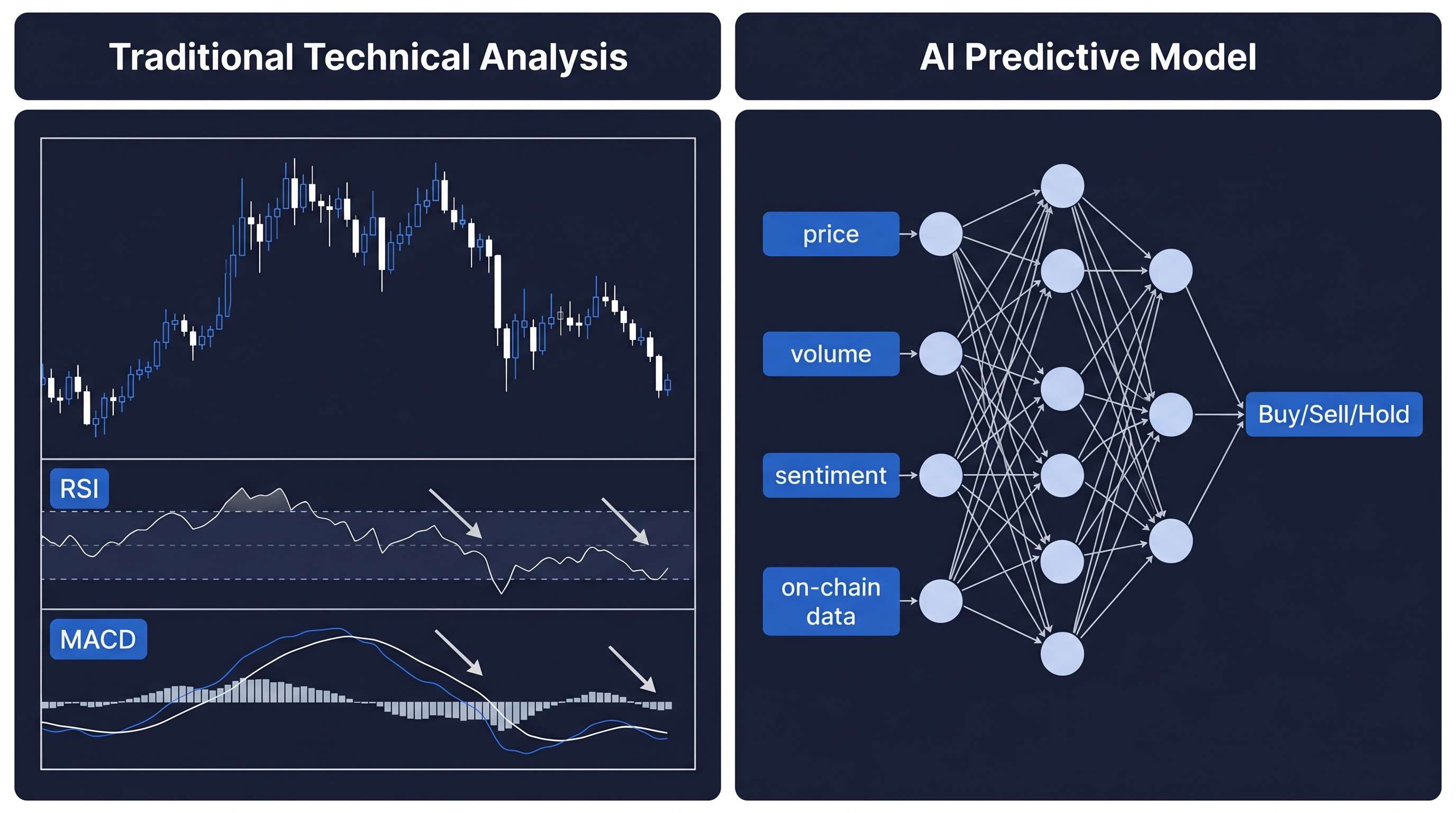
The Architecture of AI Trading Models: An Overview

Not all AI models are created equal, and choosing the right architecture for the right problem is the first decision every algo trader must make. In the context of crypto trend prediction, three model families dominate the landscape:

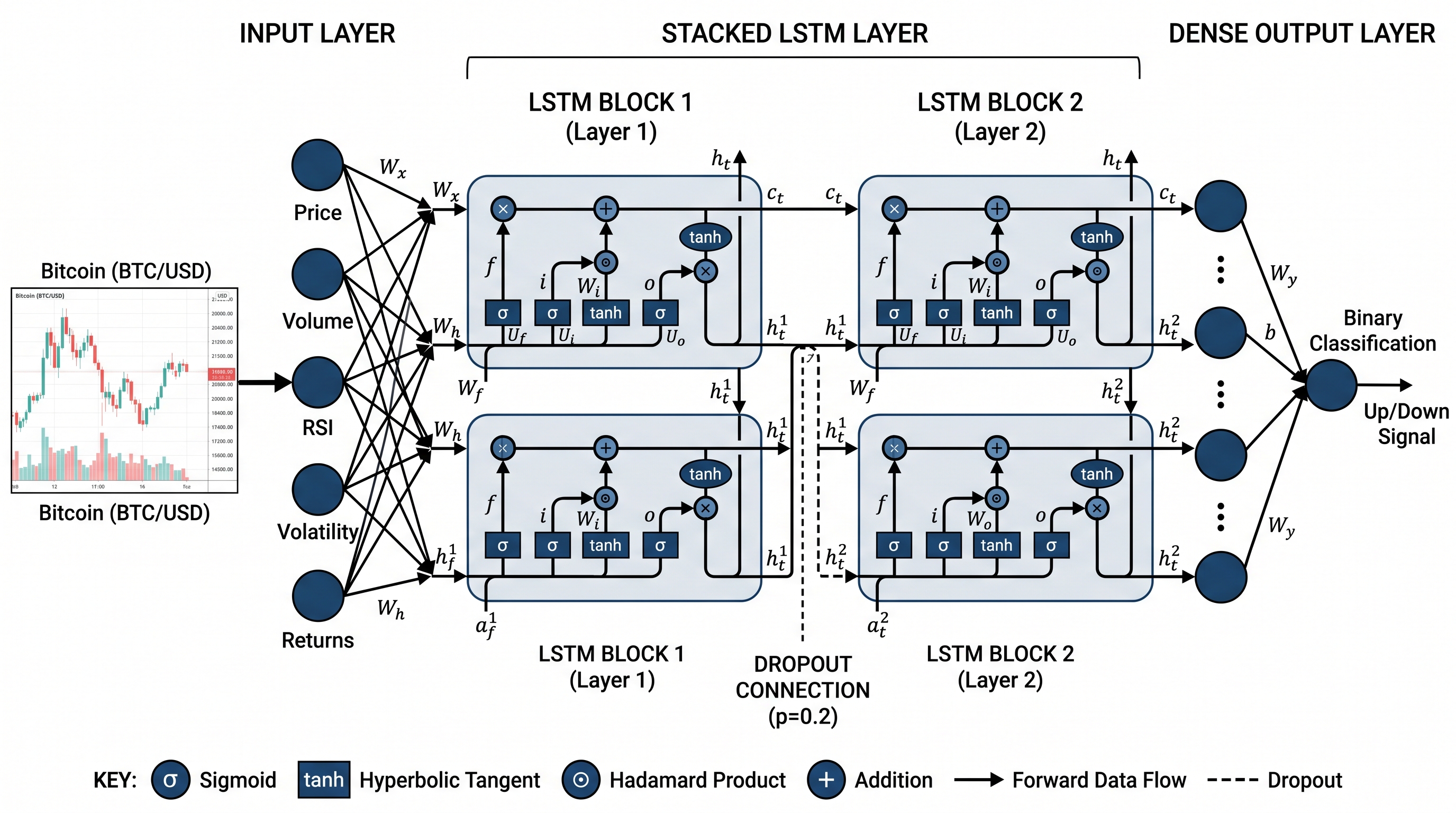
1. Recurrent Neural Networks and LSTM

Long Short-Term Memory networks, commonly abbreviated as LSTMs, are a specialized form of recurrent neural network (RNN) designed to learn from sequential data. Price time series are, by definition, sequential — each observation is meaningfully connected to what came before it. LSTMs were built to capture exactly these kinds of long-range temporal dependencies.

The key innovation of LSTM over standard RNNs is its gating mechanism. A standard RNN suffers from a problem known as the vanishing gradient — gradients used during training shrink exponentially as they propagate backward through time, making it nearly impossible for the model to learn from distant past events. LSTMs solve this with three gates — the input gate, the forget gate, and the output gate — that regulate what information is retained, updated, or discarded at each time step.

Mathematically, the LSTM cell state update is governed by:

Where:

In plain English: the forget gate decides how much of the previous cell state to keep. The input gate decides how much of the new candidate values to write into the cell state. The output gate determines what the next hidden state will look like. This combination allows LSTMs to remember trends that developed dozens of time steps ago while still being sensitive to recent price action.

2. Transformer-Based Models

Originally developed for natural language processing, transformer architectures have migrated into financial time series prediction with impressive results. Unlike LSTMs, transformers use a self-attention mechanism that allows every position in a sequence to attend to every other position simultaneously — eliminating the sequential bottleneck of RNNs entirely.

The attention score between two positions is calculated as:

Where Q, K, and V represent query, key, and value matrices, and is the dimension of the key vectors. The scaling factor prevents the dot products from growing too large, which would push the softmax function into regions with vanishingly small gradients.

For crypto trend prediction, transformers excel when trained on multivariate input — simultaneously processing price data, volume, funding rates, and sentiment scores across different timeframes.

3. Gradient Boosting Models: XGBoost and LightGBM

While neural networks capture the popular imagination, ensemble tree methods remain the workhorses of quantitative finance. XGBoost and LightGBM are gradient boosting frameworks that build decision trees sequentially, with each tree correcting the residual errors of the previous one.

These models are particularly powerful when the input features are hand-engineered — meaning when you have already extracted meaningful signals like rolling volatility, RSI divergence, or funding rate momentum before feeding them into the model. They train faster than deep learning models, are easier to interpret, and often outperform neural networks on smaller datasets.

Building a Bitcoin Price Prediction Model with LSTM in Python

Theory is useful. Code is better. Let us walk through building an LSTM model to predict Bitcoin price direction using historical OHLCV data.

Step 1: Data Collection and Preparation

We will use the ccxt library to pull historical data from Binance, and pandas for preprocessing.

1import ccxt
2import pandas as pd
3import numpy as np

from sklearn.preprocessing import MinMaxScaler

1# Initialize exchange
2exchange = ccxt.binance()
3
4# Fetch OHLCV data for BTC/USDT — 1-hour candles
5ohlcv = exchange.fetch_ohlcv('BTC/USDT', timeframe='1h', limit=2000)
6
7# Convert to DataFrame
8df = pd.DataFrame(ohlcv, columns=['timestamp', 'open', 'high', 'low', 'close', 'volume'])
9df['timestamp'] = pd.to_datetime(df['timestamp'], unit='ms')
10df.set_index('timestamp', inplace=True)
11
12print(df.tail())

This gives you a clean DataFrame with 2,000 hourly candles. The next step is feature engineering — transforming raw OHLCV data into inputs the model can learn from.

Step 2: Feature Engineering

Raw price data alone is not sufficient for a robust model. We add technical indicators as derived features.

1# Returns
2df['returns'] = df['close'].pct_change()
3
4# Log returns — preferred for modeling due to symmetry
5df['log_returns'] = np.log(df['close'] / df['close'].shift(1))
6
7# Rolling volatility (annualized)
8df['volatility'] = df['log_returns'].rolling(window=24).std() * np.sqrt(8760)
9
10# RSI
11def compute_rsi(series, period=14):
12delta = series.diff()
13gain = delta.clip(lower=0).rolling(window=period).mean()
14loss = -delta.clip(upper=0).rolling(window=period).mean()
15rs = gain / loss
16return 100 - (100 / (1 + rs))
17
18df['rsi'] = compute_rsi(df['close'])
19
20# Drop NaN rows
21df.dropna(inplace=True)

The annualized volatility formula applied here is:

Where 8760 is the number of hours in a year — because crypto markets run continuously, unlike equity markets which use 252 trading days.

Step 3: Sequence Generation and Train/Test Split

LSTMs require input in the form of fixed-length sequences. We create overlapping windows of historical data to serve as training examples.

features = ['close', 'volume', 'returns', 'volatility', 'rsi']

scaler = MinMaxScaler()

1scaled_data = scaler.fit_transform(df[features])
2
3SEQ_LEN = 48  # 48-hour lookback window
4
5def create_sequences(data, seq_len):

X, y = [], []

for i in range(len(data) - seq_len):

X.append(data[i:i + seq_len])

y.append(1 if data[i + seq_len][0] > data[i + seq_len - 1][0] else 0)

1return np.array(X), np.array(y)

X, y = create_sequences(scaled_data, SEQ_LEN)

split = int(0.8 * len(X))

X_train, X_test = X[:split], X[split:]

y_train, y_test = y[:split], y[split:]

The label here is binary: 1 if the next hourly close is higher than the current close, 0 otherwise. This frames the problem as directional classification rather than price regression — a framing that tends to produce more actionable signals for trading.

Step 4: Model Architecture and Training

1import tensorflow as tf

from tensorflow.keras.models import Sequential

from tensorflow.keras.layers import LSTM, Dense, Dropout

model = Sequential([

LSTM(128, return_sequences=True, input_shape=(SEQ_LEN, len(features))),

Dropout(0.2),

LSTM(64, return_sequences=False),

Dropout(0.2),

Dense(32, activation='relu'),

Dense(1, activation='sigmoid')

])

model.compile(optimizer='adam', loss='binary_crossentropy', metrics=['accuracy'])

history = model.fit(

X_train, y_train,

epochs=30,

batch_size=64,

validation_data=(X_test, y_test),

1shuffle=False  # Critical — preserve time ordering
2)

A few design decisions worth noting. The Dropout layers with a rate of 0.2 randomly deactivate 20% of neurons during training, a regularization technique that reduces overfitting. The shuffle=False argument is critically important — shuffling time series data would contaminate your training set with future information, producing unrealistically optimistic results.

Integrating Sentiment Analysis: The Signal That Price Alone Cannot See

A model trained purely on price data is, by definition, reactive. It can only learn from what the market has already priced in. To gain a genuine edge, you need inputs that reflect market sentiment before it is fully reflected in price.

Crypto markets are uniquely susceptible to narrative-driven movements. The Fear and Greed Index, Twitter/X sentiment scores, Reddit discussion volume, and news headline sentiment have all demonstrated statistically significant predictive power in peer-reviewed studies of crypto returns.

Using the Alternative.me Fear and Greed Index

The Fear and Greed Index is a composite score ranging from 0 (Extreme Fear) to 100 (Extreme Greed), calculated daily from volatility, market momentum, social media, surveys, dominance, and trends data.

1import requests
2
3def fetch_fear_greed(limit=200):
4url = f"https://api.alternative.me/fng/?limit={limit}"
5response = requests.get(url)
6data = response.json()['data']
7fg_df = pd.DataFrame(data)
8fg_df['timestamp'] = pd.to_datetime(fg_df['timestamp'].astype(int), unit='s')
9fg_df['value'] = fg_df['value'].astype(int)
10fg_df.set_index('timestamp', inplace=True)
11fg_df = fg_df[['value']].rename(columns={'value': 'fear_greed'})
12return fg_df.sort_index()
13
14fg_df = fetch_fear_greed()
15print(fg_df.tail())

Once fetched, this feature can be merged with your OHLCV DataFrame and included as an additional input to your LSTM or XGBoost model. Empirically, adding sentiment scores as lagged features — meaning today's Fear and Greed score predicting tomorrow's return — reduces look-ahead bias while preserving predictive value.

On-Chain Data as a Predictive Layer

Beyond sentiment, on-chain metrics provide a uniquely crypto-native layer of information. Metrics such as the Network Value to Transactions ratio, active address count, exchange inflow/outflow volume, and miner wallet balances carry information about fundamental network activity that price alone cannot capture.

The NVT ratio is conceptually similar to the price-to-earnings ratio in equities:

A high NVT suggests the network is overvalued relative to its usage — historically a bearish signal. A low NVT suggests the opposite. Incorporating this into a feature matrix alongside price-derived indicators creates a richer, multi-dimensional signal for your model.

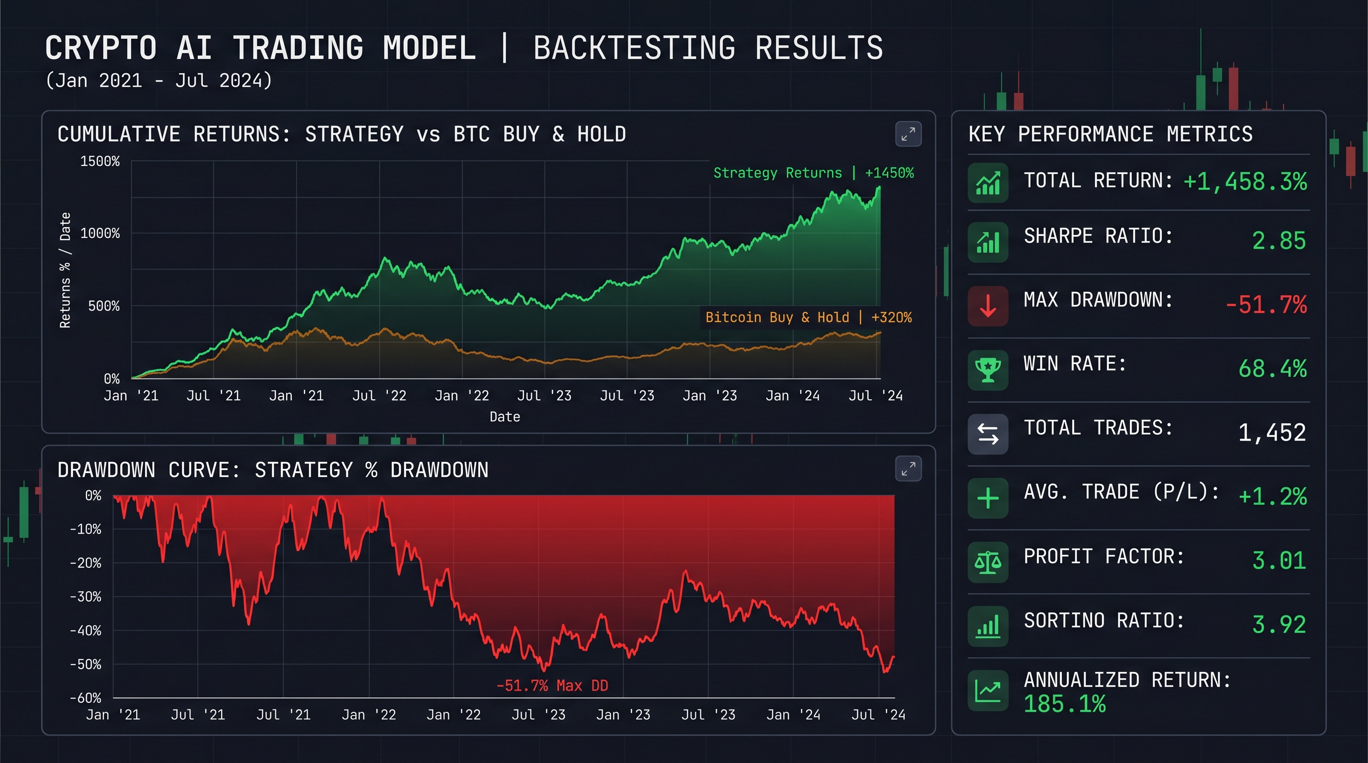
Backtesting Your AI Model: The Step Most Traders Skip

A model that performs well in training and testing on historical data is promising. A model that holds up in a rigorous backtest is worth deploying.

Backtesting is the process of simulating your model's trading decisions against historical data to estimate how it would have performed in real market conditions. The critical discipline here is avoiding lookahead bias — the inadvertent use of future information to make past predictions.

The Sharpe ratio is the most commonly used metric to evaluate risk-adjusted backtesting performance:

Where is the mean portfolio return, is the risk-free rate, and is the standard deviation of portfolio returns. A Sharpe ratio above 1.0 is generally considered acceptable; above 2.0 is excellent for a crypto strategy.

Maximum drawdown — the largest peak-to-trough decline over the backtest period — is equally important:

A strategy with a high Sharpe ratio but an 80% maximum drawdown is not deployable in practice — no trader will psychologically survive that journey.

1import vectorbt as vbt
2
3# Generate signals from model predictions
4signals = model.predict(X_test).flatten()
5buy_signal = signals > 0.55   # Buy when model confidence exceeds 55%
6sell_signal = signals < 0.45  # Sell when confidence drops below 45%
7
8# Run backtest using vectorbt
9price_series = pd.Series(
10df['close'].values[split + SEQ_LEN:],
11index=df.index[split + SEQ_LEN:]
12)
13
14portfolio = vbt.Portfolio.from_signals(

price_series,

entries=buy_signal,

exits=sell_signal,

init_cash=10000,

fees=0.001

)

1print(portfolio.stats())

The vectorbt library offers vectorized backtesting — meaning it computes all trades simultaneously rather than looping through them — making it orders of magnitude faster than traditional event-driven backtesting frameworks like Backtrader.

Common Pitfalls That Destroy AI Trading Models

Understanding what can go wrong is as valuable as knowing what to build. The following failure modes are responsible for the majority of underperforming AI trading models in production.

Overfitting to historical noise. A model with too many parameters trained on too little data will memorize the training set rather than learning generalizable patterns. The result is spectacular in-sample performance and catastrophic live trading. Always validate on out-of-sample data and walk-forward test before deploying.

Survivorship bias in training data. If your training dataset only includes cryptocurrencies that are still trading today, you have implicitly excluded every asset that failed — which constitutes the majority of historical crypto projects. This introduces a systematic upward bias into your model's expectations.

Transaction cost neglect. Even a 0.1% fee per trade — modest by most standards — compounds dramatically at high signal frequencies. A strategy that generates 5 trades per day at 0.1% per trade pays 182.5% in fees per year. Always include realistic fee assumptions in your backtest.

Non-stationarity. Financial time series are non-stationary — their statistical properties (mean, variance, autocorrelation structure) change over time. A model trained on the 2020–2021 bull market will have a distorted view of reality when deployed in the 2022–2023 bear market. Periodic retraining and regime detection are essential.

What Comes Next: Reinforcement Learning and Adaptive Models

The models covered in this post represent the current mainstream of AI-driven crypto trading — but the frontier is moving fast.

Reinforcement learning (RL) approaches treat the trading problem as a sequential decision process: an agent observes the market state, takes an action (buy, sell, hold), receives a reward (profit or loss), and updates its policy accordingly. Unlike supervised learning, which learns from labeled historical outcomes, RL learns by interacting with the environment. This allows it to adapt dynamically to regime changes in ways that static supervised models cannot.

Libraries like stable-baselines3 and FinRL make it increasingly practical to experiment with RL-based trading agents without a background in control theory or academic reinforcement learning literature.

The next evolution beyond that is multi-agent architectures — where ensembles of specialized models handle different market regimes simultaneously, routing signal generation through an orchestration layer that weights each model's contribution based on detected market conditions. This is, broadly, how the most sophisticated quantitative funds currently operate.

Key Takeaways

• LSTM networks are the dominant architecture for sequential price data, using gating mechanisms to capture long-range temporal dependencies that standard indicators miss.
• Transformer models offer parallel computation advantages and excel on multivariate inputs across multiple timeframes.
• Sentiment data — Fear and Greed Index, on-chain metrics, and social signals — adds a predictive layer that price-only models cannot replicate.
• Rigorous backtesting with realistic fee assumptions, out-of-sample validation, and drawdown analysis is non-negotiable before deployment.
• Overfitting, survivorship bias, and non-stationarity are the three most common causes of AI trading model failure in production.

Conclusion: The Edge Is in the Architecture

The most important insight from this entire post is this: AI does not give you an edge simply by being AI. A poorly designed LSTM trained on biased data with no transaction cost accounting will lose money faster than the simplest rule-based system. The edge comes from disciplined architecture choices, rigorous validation, and a genuine understanding of the domain you are modeling.

The good news is that everything covered in this post — LSTM construction, sentiment integration, vectorized backtesting — is accessible to any Python-familiar trader willing to invest the time.

Your next step is to run the code blocks above on real data. Pull Bitcoin hourly candles from Binance, engineer the features, train the LSTM, and run your first backtest. Do not wait until the model is perfect. Get it running, understand its failure modes, and iterate from there.

The market is running. Your model should be too.