AI Signal Confirmation Strategy for Better Trading Accuracy

Introduction: The Problem Machine Learning Actually Solves in Trading

Most discussions of AI in trading start from the wrong direction. They frame machine learning as a system for predicting where price will go next, as if the primary challenge in trading is forecasting direction. It is not. Systematic traders with well-designed strategies already have a mechanism for generating directional signals. The primary challenge they face is not generating signals — it is separating the signals that are likely to work in the current market environment from those that are not.

This is precisely the problem machine learning is well-suited to solve. A classification model that asks "given the current market conditions, is this signal likely to produce a profitable outcome?" is a fundamentally different application from one that asks "what will price do next?" The first question has a tractable feature space, a well-defined target variable, and a use case that aligns with how experienced traders actually think about signal quality. The second is attempting to predict inherently stochastic behavior, which leads to overfitted, curve-fitted models that define most retail AI trading attempts.

This post builds an AI signal confirmation system from the ground up. You will learn how to engineer features from market data that are genuinely predictive of signal quality, how to label training data correctly without introducing look-ahead bias, how to train and validate a classification model, and how to deploy it as a real-time filter in a live trading pipeline.

The Signal Confirmation Architecture

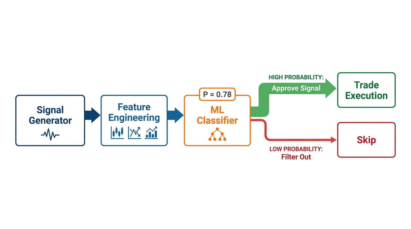
The AI confirmation system sits between the signal generator and the execution engine. It receives every signal the strategy produces, evaluates it against current market conditions, and returns a confirmation score (0–100) that represents the model's confidence that this signal will produce a profitable outcome in the current environment:

Strategy Signal → AI Confirmation Filter → Confirmed (execute) / Rejected (skip)

The model does not change the strategy's entry, stop, or target logic. It answers one question: should this particular signal, in these particular market conditions, be acted upon?

Feature Engineering for Signal Quality

The features that predict signal quality are different from the features that generate the signal itself. Signal-generating features measure directional conditions (is the trend bullish?). Signal-quality features measure environmental conditions (is the market conducive to the signal's success?):

python

1# signal_quality_features.py
2
3import pandas as pd
4import numpy as np
5
6
7def engineer_signal_quality_features(
8    ohlcv: pd.DataFrame,
9    signal_info: dict,
10) -> dict:
11    """
12    Engineers features that predict whether a trading signal will succeed.
13    
14    These features do NOT predict price direction. They predict whether
15    the current market environment is conducive to the signal's success.
16    
17    Feature categories:
18    1. Volatility Environment: Is vol expanding or contracting? Low vol
19       breakouts have lower follow-through. High vol with trend = good.
20    2. Volume Context: Is participation supporting the signal direction?
21    3. Trend Strength: Is there genuine trend, or is price oscillating?
22    4. Signal-Specific Features: How extreme is this particular signal?
23    5. Regime Features: What is the current market regime?
24    """
25    close = ohlcv["close"]
26    high = ohlcv["high"]
27    low = ohlcv["low"]
28    volume = ohlcv["volume"]
29
30    features = {}
31
32    # 1. Volatility Features
33    tr = pd.concat([
34        high - low, (high - close.shift(1)).abs(), (low - close.shift(1)).abs()
35    ], axis=1).max(axis=1)
36    atr = tr.rolling(14).mean()
37    atr_avg_50 = atr.rolling(50).mean()
38
39    features["atr_ratio"] = float(atr.iloc[-1] / atr_avg_50.iloc[-1]) \
40        if atr_avg_50.iloc[-1] > 0 else 1.0
41    features["atr_trend"] = 1 if float(atr.iloc[-1]) > float(atr.iloc[-5]) else 0
42    features["bb_width_percentile"] = compute_bbw_percentile(ohlcv)
43
44    # 2. Volume Features
45    avg_vol = float(volume.rolling(20).mean().iloc[-1])
46    features["volume_ratio"] = float(volume.iloc[-1]) / avg_vol if avg_vol > 0 else 1.0
47    features["volume_trend"] = 1 if float(volume.iloc[-3:].mean()) > \
48                               float(volume.iloc[-6:-3].mean()) else 0
49    features["obv_divergence"] = check_obv_divergence(close, volume)
50
51    # 3. Trend Strength Features
52    adx_val = compute_adx(ohlcv)
53    features["adx"] = adx_val
54    features["adx_regime"] = 2 if adx_val >= 30 else 1 if adx_val >= 20 else 0
55
56    ema_20 = float(close.ewm(span=20, adjust=False).mean().iloc[-1])
57    ema_50 = float(close.ewm(span=50, adjust=False).mean().iloc[-1])
58    features["ema_trend_strength"] = (ema_20 - ema_50) / ema_50 * 100
59
60    # 4. Signal-Specific Features
61    features["signal_direction"] = 1 if signal_info.get("direction") == "LONG" else 0
62    features["signal_strength"] = signal_info.get("strength", 0.5)
63    features["rsi_at_signal"] = compute_rsi(close)
64
65    # 5. Regime Features
66    features["session_hour"] = pd.Timestamp.now().hour  # Current UTC hour
67    features["is_weekend"] = 1 if pd.Timestamp.now().dayofweek >= 5 else 0
68
69    return features

Correct Training Data Labeling

The most common labeling mistake in trading ML is using future price change as the target without accounting for the signal's specific stop and target levels. The correct target for a signal confirmation model is whether the signal's specific outcome (hit its target or hit its stop) was profitable, using the signal's own defined risk parameters:

python

1def label_signal_outcome(
2    ohlcv: pd.DataFrame,
3    signal_entry_idx: int,
4    signal_direction: str,
5    stop_price: float,
6    target_price: float,
7    max_bars: int = 50,
8) -> int:
9    """
10    Labels whether a signal was profitable based on its specific
11    stop and target, NOT on future price change in general.
12    
13    Returns: 1 (profitable — target hit before stop),
14             0 (unprofitable — stop hit before target or time expired)
15    
16    This labeling is free of look-ahead bias because it uses the
17    signal's own defined exit parameters, which were known at entry.
18    """
19    for k in range(signal_entry_idx + 1, min(signal_entry_idx + max_bars, len(ohlcv))):
20        bar_high = float(ohlcv["high"].iloc[k])
21        bar_low = float(ohlcv["low"].iloc[k])
22
23        if signal_direction == "LONG":
24            if bar_low <= stop_price:
25                return 0
26            if bar_high >= target_price:
27                return 1
28        else:
29            if bar_high >= stop_price:
30                return 0
31            if bar_low <= target_price:
32                return 1
33
34    return 0  # Time expiration = unprofitable

XGBoost Model Training and Calibration

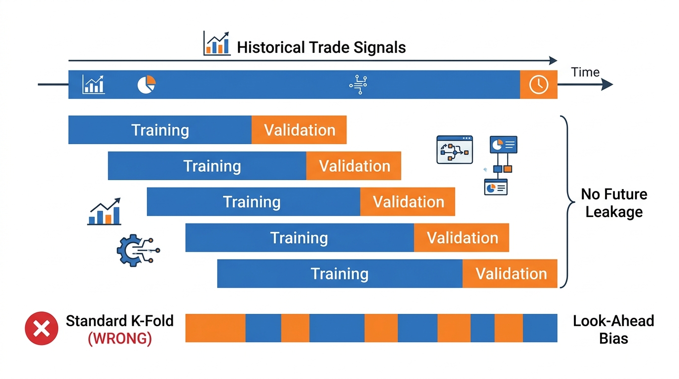
The model is an XGBoost classifier trained on historically labeled signal data with strict chronological train/test splits:

python

1import xgboost as xgb
2from sklearn.calibration import CalibratedClassifierCV
3from sklearn.model_selection import TimeSeriesSplit
4
5
6def train_confirmation_model(
7    features: np.ndarray,
8    labels: np.ndarray,
9) -> tuple:
10    """
11    Trains an XGBoost classifier for signal confirmation with
12    chronological cross-validation and probability calibration.
13    """
14    # Chronological split — NEVER shuffle financial time series
15    split_idx = int(len(features) * 0.70)
16    X_train, X_test = features[:split_idx], features[split_idx:]
17    y_train, y_test = labels[:split_idx], labels[split_idx:]
18
19    # Handle class imbalance
20    scale_pos_weight = (len(y_train) - sum(y_train)) / sum(y_train) \
21        if sum(y_train) > 0 else 1.0
22
23    model = xgb.XGBClassifier(
24        n_estimators=150,
25        max_depth=4,
26        learning_rate=0.05,
27        subsample=0.80,
28        colsample_bytree=0.80,
29        scale_pos_weight=scale_pos_weight,
30        random_state=42,
31        eval_metric="logloss",
32    )
33
34    model.fit(X_train, y_train,
35              eval_set=[(X_test, y_test)],
36              early_stopping_rounds=15,
37              verbose=False)
38
39    # Calibrate probabilities
40    calibrated = CalibratedClassifierCV(
41        estimator=model, method="isotonic", cv=5
42    )
43    calibrated.fit(X_train, y_train)
44
45    return calibrated, X_test, y_test
46
47
48def filter_signal_with_model(
49    signal: dict,
50    ohlcv: pd.DataFrame,
51    model,
52    min_confidence: float = 0.60,
53) -> dict:
54    """
55    Applies the AI confirmation filter to a trading signal.
56    Returns the signal with a confirmation_score and approval status.
57    """
58    features = engineer_signal_quality_features(ohlcv, signal)
59    feature_vector = np.array([list(features.values())])
60
61    probabilities = model.predict_proba(feature_vector)
62    confidence = float(probabilities[0][1])  # Probability of class 1 (profitable)
63
64    signal["ai_confidence"] = round(confidence, 4)
65    signal["ai_approved"] = confidence >= min_confidence
66    signal["position_multiplier"] = round(
67        min(1.0, confidence * 1.5), 2
68    ) if confidence >= min_confidence else 0.0
69
70    return signal

The calibrated probability serves two purposes: it determines whether the signal is approved (confidence ≥ 60%), and it scales the position size (higher confidence = larger position within risk limits).

AI signal confirmation architecture: signal → features → model → approve/reject

Feature importance analysis from trained XGBoost model

Backtest: strategy performance with and without AI confirmation filter

Confirmation model calibration curve and reliability diagram

Key Takeaways

AI signal confirmation solves a different problem than price prediction. The model asks "will this specific signal succeed in this specific environment?", not "where will price go?" This is a tractable classification problem with well-defined target labels
Training labels must be derived from each signal's specific stop and target levels, not from generic future price change. A signal that would have hit its 1.5 ATR target is successful regardless of what price did afterward
Chronological train/test splits are mandatory. Random shuffling of financial time series data leaks future information into training and produces catastrophic overfitting
Probability calibration converts raw model scores into actual empirical probabilities. After calibration, a 75% confidence prediction should be correct approximately 75% of the time — essential for position sizing
The model serves as a filter, not a replacement. The underlying strategy still generates signals using its own logic. The AI layer determines which of those signals to act upon based on environmental conditions

Conclusion

The AI signal confirmation strategy demonstrates the correct application of machine learning to systematic trading: not as a replacement for strategy logic, but as an environmental filter that evaluates whether current market conditions are conducive to the strategy's success. The model learns from historical signal outcomes which features discriminate between conditions where the strategy performs well and conditions where it underperforms.

The most important operational consideration is model retraining frequency. Market conditions evolve, and a model trained on data from six months ago may have degraded accuracy on current conditions. Implement a monthly retraining cycle that incorporates the most recent month of signal outcomes, and monitor the model's calibration curve to detect when its probability estimates begin to drift from actual outcomes.

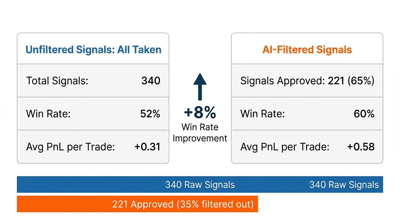
The integration is straightforward: the model sits between the signal generator and the execution engine. Every signal passes through the filter. Approved signals are executed (with position sizing scaled by confidence). Rejected signals are logged but not acted upon. The filter adds approximately zero latency to the trading pipeline while providing a measurable improvement in signal quality.