AI and Price Action Strategy for Smarter Trading Decisions

Introduction: When the Pattern Recognizer Becomes the Pattern

In 2016, DeepMind's AlphaGo defeated the world Go champion using deep neural networks and reinforcement learning. The significance for traders was not the victory itself but the mechanism: the model had learned to recognize patterns in board states that human experts had spent decades systematically studying, and it found additional patterns that no human had explicitly identified. It did not play by the rules of established Go theory. It discovered new theory.

Price action in financial markets is structurally analogous. A price chart is a high-dimensional state space where every bar encodes information about supply and demand, participant psychology, and order flow dynamics. Human traders have identified repeating patterns — head and shoulders, order blocks, fair value gaps, consolidation breakouts. These patterns have edge. But the human capacity to recognize them is bounded by cognitive limitations: we process one chart at a time, we are influenced by recency bias, and we cannot simultaneously evaluate hundreds of variables across thousands of assets.

Machine learning removes these constraints. A well-designed model can evaluate pattern recognition tasks across thousands of assets simultaneously, weight features by their historical predictive power rather than visual salience, and generate calibrated probability estimates.

This article explains how to combine AI and price action analysis into a unified trading framework: feature engineering from price action concepts, training a classifier to predict directional outcomes, calibrating and validating the model to avoid overfitting, and integrating model outputs into an executable trading system in Python.

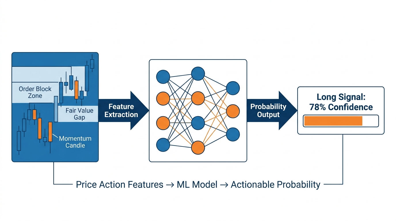
Why Price Action Features Are Ideal for Machine Learning

Feature engineering converts raw data into structured numerical representations. The quality of features determines the ceiling of model performance more than the choice of algorithm. Good features contain genuine predictive information; poor features add noise.

Price action concepts are exceptionally well-suited as ML features for three reasons:

Dimensionality meaningful: Each concept measures a specific, interpretable aspect of market behavior. An order block distance feature measures how far price is from a known institutional interest level. An ATR ratio measures whether volatility is elevated or compressed. These features have semantic content that helps the model generalize rather than memorize.

Scale-independent when normalized: An order block 2% away from current price carries the same structural meaning whether Bitcoin is at $10,000 or$70,000. Normalizing features as fractions or multiples of ATR ensures the model learns patterns that generalize across price levels and assets.

Multi-timeframe encoding simultaneously: A single feature vector can include EMA relationships from multiple periods, Fibonacci retracement positions, VWAP deviation, and volatility regime classification — allowing the model to identify complex conditional patterns that would be laborious to define as explicit rules but are learnable from labeled data.

Feature Extraction Framework

The framework transforms raw OHLCV data and indicator outputs into structured feature vectors for each bar:

1import math
2import statistics
3from typing import Optional
4
5def compute_ema(prices: list, period: int) -> Optional[float]:
6    if len(prices) < period:
7        return None
8    alpha = 2 / (period + 1)
9    ema = sum(prices[:period]) / period
10    for p in prices[period:]:
11        ema = alpha * p + (1 - alpha) * ema
12    return ema
13
14def compute_rsi(closes: list, period: int = 14) -> Optional[float]:
15    if len(closes) < period + 1:
16        return None
17    deltas = [closes[i] - closes[i-1] for i in range(1, len(closes))]
18    gains = [max(d, 0) for d in deltas]
19    losses = [abs(min(d, 0)) for d in deltas]
20    avg_gain = sum(gains[:period]) / period
21    avg_loss = sum(losses[:period]) / period
22    for i in range(period, len(gains)):
23        avg_gain = (avg_gain * (period - 1) + gains[i]) / period
24        avg_loss = (avg_loss * (period - 1) + losses[i]) / period
25    if avg_loss == 0:
26        return 100.0
27    return 100 - (100 / (1 + avg_gain / avg_loss))
28
29def compute_atr(highs: list, lows: list, closes: list,
30                period: int = 14) -> Optional[float]:
31    if len(closes) < period + 1:
32        return None
33    trs = []
34    for i in range(1, len(closes)):
35        tr = max(
36            highs[i] - lows[i],
37            abs(highs[i] - closes[i-1]),
38            abs(lows[i] - closes[i-1])
39        )
40        trs.append(tr)
41    return statistics.mean(trs[-period:]) if len(trs) >= period else None
42
43def compute_vwap(highs: list, lows: list, closes: list,
44                 volumes: list) -> Optional[float]:
45    if len(closes) == 0 or sum(volumes) == 0:
46        return None
47    typical_prices = [(h + l + c) / 3 for h, l, c in zip(highs, lows, closes)]
48    cum_pv = sum(tp * v for tp, v in zip(typical_prices, volumes))
49    cum_vol = sum(volumes)
50    return cum_pv / cum_vol

Feature Categories Extracted Per Bar

Trend and Momentum Features:

• EMA ratios (EMA_9 / EMA_21, EMA_20 / EMA_50)
• RSI value and RSI regime (oversold < 30, neutral 30–70, overbought > 70)
• MACD line, signal line, and histogram values

Volatility Features:

• ATR ratio (current ATR / ATR 20 periods ago)
• Bollinger Band width and position within bands
• Volatility regime classification (compression, normal, expansion)

Structural Features:

• Distance to nearest order block (normalized by ATR)
• Distance to nearest fair value gap
• Fibonacci retracement position (0.382, 0.5, 0.618, 0.786)
• VWAP deviation (percentage above/below VWAP)

Volume Features:

• Volume ratio (current volume / 20-period rolling average)
• Volume trend (5-period volume MA vs 20-period volume MA)
• Relative volume percentile

Multi-Timeframe Features:

• Higher timeframe trend classification (bullish/bearish based on EMA alignment)
• Higher timeframe ADX value
• Multi-timeframe alignment score

Target Variable Definition

The prediction target must be mathematically precise and aligned with how the signal will be used in trading:

1def define_target(closes: list, idx: int, horizon: int = 5,
2                  threshold_pct: float = 0.005) -> int:
3    """
4    Define the target variable for supervised learning.
5    1 = bullish (price increases by threshold within horizon)
6    0 = neutral/ ranging
7    -1 = bearish (price decreases by threshold within horizon)
8    """
9    if idx + horizon >= len(closes):
10        return None
11    future_close = closes[idx + horizon]
12    current_close = closes[idx]
13    pct_change = (future_close - current_close) / current_close
14
15    if pct_change > threshold_pct:
16        return 1
17    elif pct_change < -threshold_pct:
18        return -1
19    else:
20        return 0

Using a horizon of 5 bars with a 0.5% threshold means the model predicts whether price will move meaningfully in a given direction within the next 5 candles. The neutral class (0) prevents the model from being forced to make directional predictions during ranging periods where no edge exists.

Model Architecture and Training

Choice of Algorithm

For tabular price action features with strong structural relationships, tree-based ensemble methods consistently outperform neural networks on out-of-sample data:

XGBoost is the primary recommendation for production systems. It handles missing values natively, is robust to uninformative features, provides built-in feature importance metrics, trains quickly on CPU, and has excellent out-of-box performance with minimal hyperparameter tuning.

Random Forest is a simpler alternative that is less prone to overfitting and requires less hyperparameter tuning, making it ideal for initial prototyping before moving to XGBoost.

1import xgboost as xgb
2from sklearn.model_selection import train_test_split
3from sklearn.metrics import classification_report
4
5# Prepare feature matrix and target vector
6X = feature_vectors  # shape: (n_samples, n_features)
7y = targets          # shape: (n_samples,)
8
9# Chronological split (NEVER shuffle time-series data randomly)
10split_idx = int(len(X) * 0.7)
11X_train, X_test = X[:split_idx], X[split_idx:]
12y_train, y_test = y[:split_idx], y[split_idx:]
13
14# Handle class imbalance with scale_pos_weight
15unique, counts = np.unique(y_train, return_counts=True)
16class_weights = {c: len(y_train) / (len(unique) * count)
17                 for c, count in zip(unique, counts)}
18
19model = xgb.XGBClassifier(
20    n_estimators=200,
21    max_depth=5,
22    learning_rate=0.05,
23    subsample=0.8,
24    colsample_bytree=0.8,
25    scale_pos_weight=class_weights.get(1, 1.0),
26    random_state=42,
27    eval_metric='mlogloss'
28)
29
30model.fit(X_train, y_train,
31          eval_set=[(X_test, y_test)],
32          early_stopping_rounds=20,
33          verbose=False)
34
35# Evaluate
36y_pred = model.predict(X_test)
37print(classification_report(y_test, y_pred))

Critical: Chronological Split, Never Random

Financial data has temporal dependence. Randomly shuffling samples between train and test sets leaks future information into training and produces catastrophically misleading backtest results. Always split chronologically: train on earlier periods, test on later periods.

Addressing Class Imbalance

Trading datasets are typically imbalanced — strong trends are rarer than ranging conditions. Address this with scale_pos_weight in XGBoost, SMOTE oversampling (applied within each training fold only), or class-weighted loss functions.

Probability Calibration

Raw model outputs are not true probabilities — they are uncalibrated scores. A prediction of 0.75 may only be correct 60% of the time. Calibration maps raw scores to actual empirical probabilities:

1from sklearn.calibration import CalibratedClassifierCV
2
3calibrated_model = CalibratedClassifierCV(
4    estimator=model,
5    method='isotonic',
6    cv=5  # 5-fold cross-validation on training data
7)
8calibrated_model.fit(X_train, y_train)
9
10# Now predict_proba returns calibrated probabilities
11probabilities = calibrated_model.predict_proba(X_test)

After calibration, when the model says 78% confidence, it should be correct approximately 78% of the time — making it usable for position sizing and risk management decisions.

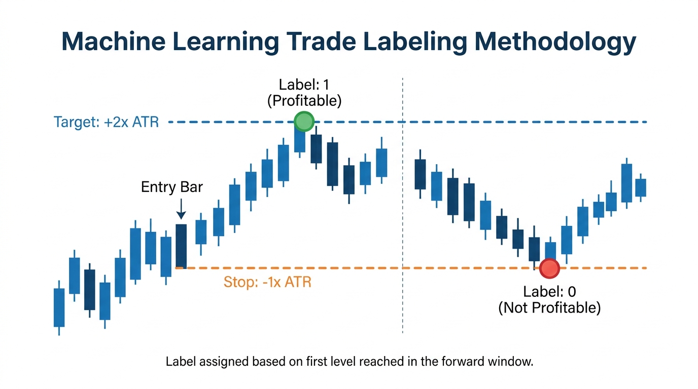
Validation: Purged Walk-Forward Testing

Standard cross-validation underestimates error in financial time series because adjacent samples are correlated. Purged walk-forward validation addresses this by training on a rolling window of historical data, testing on the immediately following out-of-sample period, purging samples that overlap between train and test sets, and never using future data for training:

1def purged_walk_forward(X, y, train_window=500, test_window=100,
2                         purge_window=10):
3    results = []
4    start = 0
5
6    while start + train_window + test_window <= len(X):
7        train_end = start + train_window
8        test_start = train_end + purge_window  # Purge overlap
9        test_end = test_start + test_window
10
11        X_tr = X[start:train_end]
12        y_tr = y[start:train_end]
13        X_te = X[test_start:test_end]
14        y_te = y[test_start:test_end]
15
16        model = xgb.XGBClassifier(n_estimators=200, max_depth=5,
17                                   learning_rate=0.05)
18        model.fit(X_tr, y_tr)
19        y_pred = model.predict(X_te)
20
21        results.append({
22            'train_period': (start, train_end),
23            'test_period': (test_start, test_end),
24            'accuracy': (y_pred == y_te).mean()
25        })
26
27        start += test_window  # Roll forward
28
29    return results

Trading System Integration

Signal Generation Framework

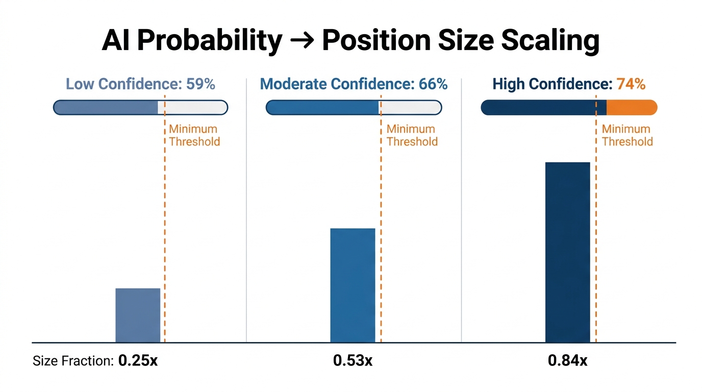
The calibrated model probability thresholds determine entry decisions:

1def generate_signal(probabilities: dict, config: dict) -> dict:
2    """
3    Convert model probabilities into actionable trading signals.
4    config specifies minimum confidence thresholds for each action.
5    """
6    long_conf = probabilities.get('long', 0)
7    short_conf = probabilities.get('short', 0)
8
9    if long_conf >= config['min_long_confidence']:
10        action = 'long'
11        confidence = long_conf
12    elif short_conf >= config['min_short_confidence']:
13        action = 'short'
14        confidence = short_conf
15    else:
16        action = 'neutral'
17        confidence = max(long_conf, short_conf)
18
19    return {
20        'action': action,
21        'confidence': confidence,
22        'position_size_multiplier': confidence  # Kelly-inspired scaling
23    }

Regime Gating

Even a well-calibrated model should be gated by market regime. When ADX is below 20 and volatility is compressing, the model's edge may disappear. Implement a regime gate that only allows signals when market conditions match the training distribution:

1def regime_gate(features: dict) -> bool:
2    """Prevent trading when market regime doesn't match training regime."""
3    adx = features.get('adx', 0)
4    atr_ratio = features.get('atr_ratio', 1.0)
5
6    # Model was trained on trending, non-extreme volatility data
7    if adx < 20:
8        return False  # Ranging market — model edge is weak
9    if atr_ratio > 3.0:
10        return False  # Extreme volatility — out of distribution
11
12    return True

Monitoring and Maintenance

Model performance degrades over time — this is inevitable as market regimes shift. Implement a monitoring system:

Daily metrics: Track signal distribution (what percentage of signals are long, short, neutral), average confidence scores, and signal frequency. Drift in any of these indicates the model is seeing data unlike its training distribution.

Weekly metrics: Track realized win rate vs expected win rate (from calibration curve), actual Sharpe ratio vs backtest Sharpe ratio, and profit factor. Divergence between expected and realized metrics triggers investigation.

Monthly retraining: Retrain the model on an expanded dataset that includes the most recent month of labeled data. Compare new model performance to the deployed model on a shared test set. Only deploy if the new model shows statistically significant improvement.

Key Takeaways

• Price action features are ideal for machine learning because they are dimensionally meaningful, scale-independent when ATR-normalized, and encode multi-timeframe information simultaneously
• Feature extraction should produce structured vectors spanning trend, momentum, volatility, structural, volume, and multi-timeframe dimensions — typically 30–50 features per bar
• Tree-based ensemble methods (XGBoost, Random Forest) consistently outperform neural networks on tabular price action data with strong structural relationships
• Never randomly shuffle time-series data — always use chronological train/test splits and purged walk-forward validation
• Probability calibration (isotonic or Platt scaling) is essential — raw model scores are not real probabilities and should not be used for position sizing
• Implement regime gating to prevent trading when market conditions don't match the training distribution
• Monitor signal distribution, confidence calibration, and realized vs expected performance metrics continuously
• Retrain monthly on expanded data and only deploy new models that show statistically significant improvement

Conclusion

The integration of AI and price action is not about replacing human trading intuition with black-box predictions. It is about amplifying systematic pattern recognition to a scale and consistency that human cognition cannot replicate. The edge comes from the same price action concepts covered throughout this series — order blocks, fair value gaps, momentum confirmation, volatility regimes. What machine learning adds is the ability to weight these features by their actual historical predictive power, combine them into conditional patterns too complex for explicit rules, and produce calibrated probability estimates that can drive systematic position sizing.

The framework presented here is a starting point for production deployment. Build the feature extraction pipeline first and validate that your features contain genuine predictive information before training any model. Train on multiple years of data spanning bull, bear, and ranging regimes. Calibrate probabilities. Validate with purged walk-forward testing. Deploy with conservative confidence thresholds and strict regime gating. Monitor continuously.

The market evolves. Your model should too. A strategy that is systematically retrained and monitored will outlast a strategy that is built once and deployed indefinitely.