AI Prediction Errors in Trading Systems: What They Are, Why They Happen, and How to Fix Them

Introduction: The Model That Destroyed a Fund

In 2007, a quantitative hedge fund running sophisticated statistical arbitrage strategies experienced what became known as the "Quant Quake" — a period of several days in August where dozens of well-backtested, heavily optimized models simultaneously collapsed, generating catastrophic losses across the industry. The models had not been hacked. The data feeds had not failed. The mathematics was not wrong.

The models had simply encountered something their training data could not have prepared them for: a correlated unwinding of positions across the entire quant industry that created market conditions statistically unlike anything in the historical record. Every prediction they made was wrong. Not occasionally — systematically wrong, at the worst possible moment.

Here is the counterintuitive truth that every AI-driven algo trader needs to internalize early: the danger of an AI prediction error is not just that it costs you money on a single trade. It is that AI models fail coherently — they make the same kind of wrong prediction repeatedly, in the same market conditions, in ways that compound losses rather than randomly distribute them.

Understanding exactly how and why AI prediction errors occur in trading systems is not a defensive skill. It is the skill that separates traders who survive long enough to compound from those who blow up on their first regime change.

In this post, you will learn the taxonomy of AI prediction errors — from the obvious to the deeply subtle — the mathematical diagnostics that reveal them before they destroy live capital, and the practical Python tools to detect, monitor, and mitigate each error type in a working trading system. If you build AI trading models and you leave before the end, you are leaving without the knowledge most likely to save your account.

The Taxonomy of AI Prediction Errors in Trading

Not all prediction errors are created equal. Some are statistical. Some are structural. Some are invisible in backtesting but catastrophic in live deployment. The first step toward managing prediction errors is knowing which type you are dealing with — because the diagnosis determines the remedy.

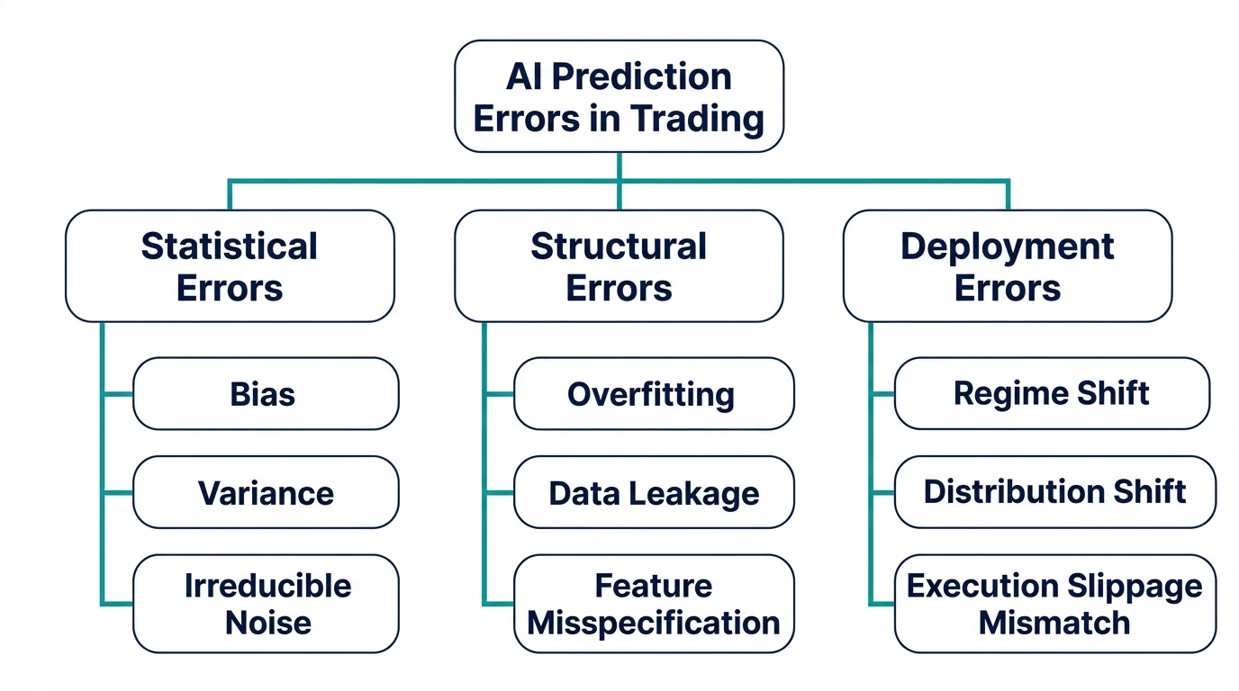
Statistical Errors: Bias, Variance, and Noise

Every prediction error can be decomposed into three fundamental components. This decomposition, known as the bias-variance-noise tradeoff, is the foundational diagnostic framework for understanding model performance.

For a model making prediction $\hat{y}$ of a true value $y$, the expected prediction error is:

Bias is the systematic error introduced by the model's assumptions. A model that assumes linear relationships in a nonlinear market will consistently predict in the wrong direction — not randomly, but predictably. High bias is the signature of underfitting — a model too simple to capture the true structure of the data.

Variance is the model's sensitivity to fluctuations in the training data. A high-variance model changes its predictions dramatically when trained on slightly different data samples — it has learned the noise in its training set rather than the underlying signal. High variance is the signature of overfitting.

Irreducible noise — represented by $\sigma_{\epsilon}^{2}$ — is the portion of prediction error that no model can eliminate, because it reflects genuine randomness in the process being predicted. In financial markets, this component is substantial. Markets are not deterministic, and any model that appears to predict with near-zero error on historical data has almost certainly memorized noise rather than learned signal.

The practical implication for trading model development is direct: you are always navigating a tradeoff. Reducing bias by adding model complexity increases variance. The goal is not to minimize one or the other, but to find the complexity level at which total out-of-sample error is minimized.

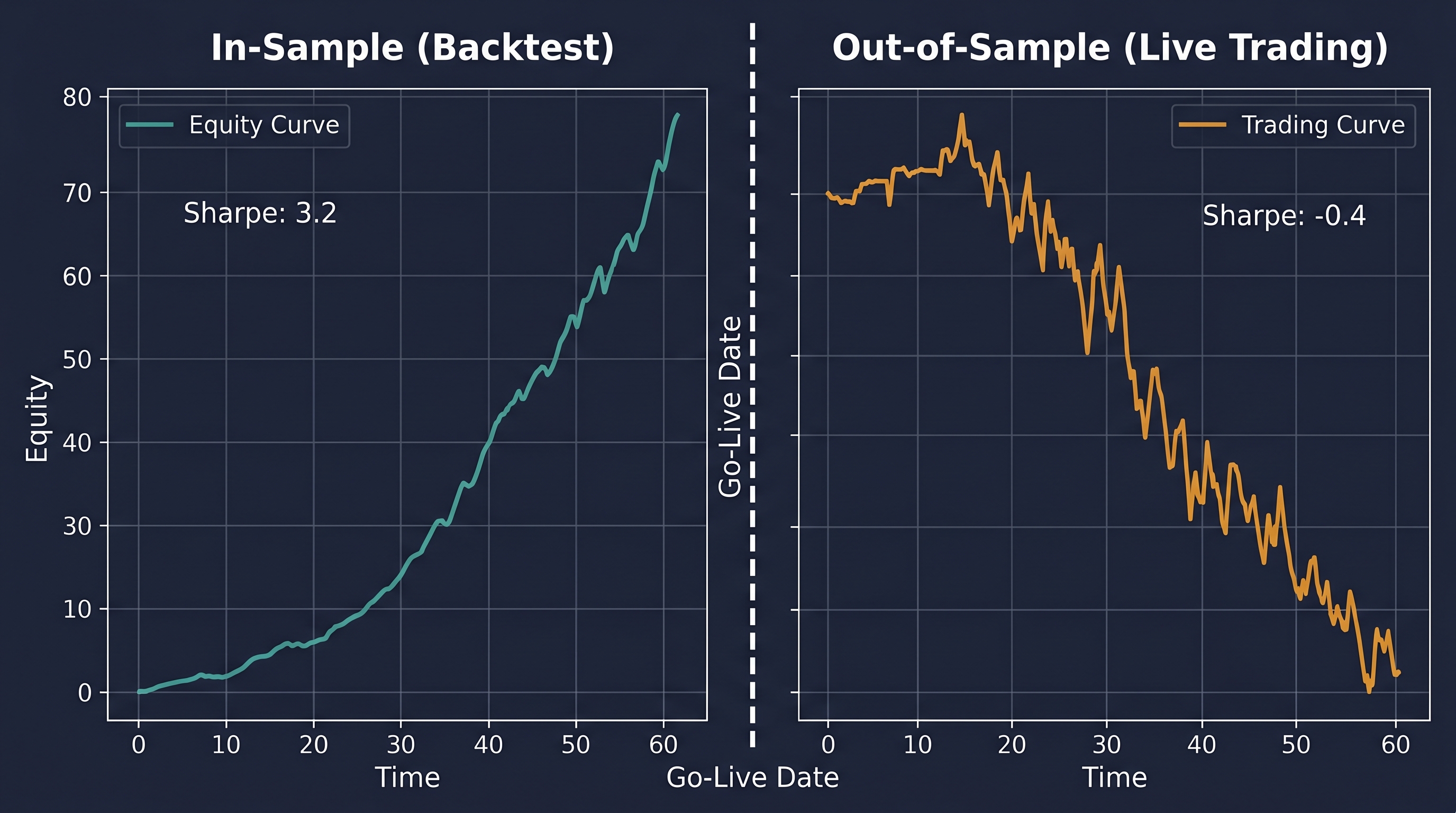
Overfitting: The Error That Looks Like Success

Overfitting is the most common and most dangerous AI prediction error in trading systems, precisely because it is invisible in backtesting. A model that has overfit its training data produces a backtest that looks exceptional — high Sharpe ratio, low drawdown, consistent returns. And then it fails completely in live trading.

The mechanism is straightforward. A sufficiently complex model trained on historical market data will eventually memorize every idiosyncratic fluctuation in that data — random noise events, one-off reactions to specific news, microstructure artifacts from specific exchanges. It mistakes these for repeatable patterns and incorporates them into its prediction function. When those exact conditions never recur in live markets, the model's predictions are worse than random on precisely the scenarios where it is most confident.

Diagnosing Overfitting with Learning Curves

The most reliable diagnostic tool for overfitting is the learning curve — a plot of training loss and validation loss as a function of training data size or training epochs.

1import numpy as np
2import pandas as pd
3import matplotlib.pyplot as plt

from sklearn.ensemble import RandomForestClassifier

from sklearn.model_selection import learning_curve

1# Assumes X and y are already prepared feature matrix and binary target

train_sizes, train_scores, val_scores = learning_curve(

estimator=RandomForestClassifier(n_estimators=200, max_depth=5, random_state=42),

X=X,

y=y,

1train_sizes=np.linspace(0.1, 1.0, 10),
2cv=5,

scoring='roc_auc',

n_jobs=-1

)

1train_mean = train_scores.mean(axis=1)
2val_mean = val_scores.mean(axis=1)
3train_std = train_scores.std(axis=1)
4val_std = val_scores.std(axis=1)
5
6plt.figure(figsize=(10, 6))
7plt.plot(train_sizes, train_mean, label='Training AUC', color='teal')
8plt.fill_between(train_sizes, train_mean - train_std, train_mean + train_std, alpha=0.15, color='teal')
9plt.plot(train_sizes, val_mean, label='Validation AUC', color='orange')
10plt.fill_between(train_sizes, val_mean - val_std, val_mean + val_std, alpha=0.15, color='orange')
11plt.axhline(y=0.5, linestyle='--', color='gray', label='Random Baseline')
12plt.xlabel('Training Set Size')
13plt.ylabel('ROC-AUC Score')
14plt.title('Learning Curve: Overfitting Diagnosis')
15plt.legend()
16plt.tight_layout()
17plt.show()

The gap between the training AUC and validation AUC is your overfitting signal. A large, persistent gap — where training AUC is high (above 0.75) and validation AUC remains close to 0.5 — indicates the model is memorizing the training data rather than learning generalizable patterns. The remedy is regularization: reducing model depth, adding dropout or L2 weight penalties, or reducing the number of features.

The generalization gap can be quantified directly:

A gap above 0.10 in financial models warrants immediate investigation. A gap above 0.20 means the model should not be deployed.

Data Leakage: The Invisible Contamination

If overfitting is the most common AI prediction error, data leakage is the most insidious. It is the error that produces the most convincing false signals — models that appear extraordinarily predictive in backtesting but perform at or below random chance in live trading, with no obvious explanation for the gap.

Data leakage occurs when information from outside the legitimate training window contaminates the model's learning process. There are two primary forms.

Target Leakage

Target leakage happens when features used to train the model contain information about the target variable that would not be available at prediction time. In trading, this occurs most commonly through improper use of rolling calculations.

Consider computing a 20-day rolling mean to use as a feature. If you compute this rolling mean on the full dataset before splitting into train and test, the rolling mean at day 300 will incorporate price data from days 281 through 300 — but if day 300 is in your test set and you are predicting the close of day 301, the rolling mean is legitimate. The danger arises from subtler cases: using tomorrow's open as part of today's feature set, computing volatility using today's data that would not be available until after market close, or including any derived statistic that implicitly references future data.

1# WRONG: Computes rolling mean on full dataset before split
2# The test set rows have "seen" future data through the rolling calculation
3df['rolling_mean'] = df['close'].rolling(20).mean()
4X = df[['rolling_mean', 'rsi']].values
5y = df['target'].values
6X_train, X_test = X[:split], X[split:]  # Leakage already baked in
7
8# CORRECT: Use only past data at each point
9# Ensure all features are computable from data available at prediction time
10df['rolling_mean'] = df['close'].rolling(20).mean()
11# rolling(20).mean() at row t uses rows t-19 through t — correct, as long as
12# the target is a future value (e.g., next-day return) not overlapping this window
13df['target'] = df['close'].shift(-1) > df['close']  # Next day's direction
14df.dropna(inplace=True)  # Drops incomplete rolling windows — critical

The discipline required: for every feature, explicitly trace which rows of historical data it uses. If any of those rows overlap with or postdate the target being predicted, you have leakage.

Train-Test Contamination

The second form of data leakage is contamination introduced by the evaluation methodology itself. StandardScaler fitted on the full dataset before splitting is the canonical example:

from sklearn.preprocessing import StandardScaler

1# WRONG: Scaler fitted on full dataset leaks test statistics into training
2scaler = StandardScaler()
3X_scaled = scaler.fit_transform(X)       # Mean and std computed from future test data
4X_train = X_scaled[:split]
5X_test = X_scaled[split:]
6
7# CORRECT: Scaler fitted only on training data
8scaler = StandardScaler()
9X_train = scaler.fit_transform(X[:split])  # Mean and std from training only
10X_test = scaler.transform(X[split:])       # Test data scaled using training statistics

The difference is subtle but the effect is not. Fitting the scaler on the full dataset means the scaled values in your training set have been adjusted using statistics that include future test data — giving the model information it would never have in a live deployment.

The Leakage Detection Test

A practical heuristic for detecting data leakage: if your model achieves a validation AUC above 0.65 on daily price prediction without any exotic data sources, be suspicious. Genuinely predictive AI trading signals on efficient markets rarely produce AUC values above 0.58 to 0.62 on properly held-out test data. Unusually high performance is almost always a leakage symptom, not a genuine alpha signal.

You can apply a temporal permutation test to verify:

1import numpy as np

from sklearn.ensemble import RandomForestClassifier

from sklearn.metrics import roc_auc_score

1# Train on true chronological data
2model = RandomForestClassifier(n_estimators=200, max_depth=5, random_state=42)

model.fit(X_train, y_train)

true_auc = roc_auc_score(y_test, model.predict_proba(X_test)[:, 1])

1# Shuffle target labels — a model with genuine signal should collapse
2y_train_shuffled = np.random.permutation(y_train)

model.fit(X_train, y_train_shuffled)

shuffled_auc = roc_auc_score(y_test, model.predict_proba(X_test)[:, 1])

1print(f"True AUC: {true_auc:.4f}")
2print(f"Shuffled Target AUC: {shuffled_auc:.4f}")
3print(f"Signal integrity check: {'PASS' if true_auc > shuffled_auc + 0.02 else 'INVESTIGATE'}")

If shuffling the training labels does not significantly reduce test AUC, your model is not learning a genuine temporal relationship — it is exploiting structural features of the data arrangement, which is a strong indicator of leakage.

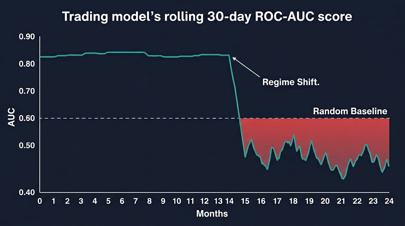
Regime Shift Errors: When the World Changes

Even a perfectly specified, properly trained, leakage-free model will eventually fail — because financial markets are non-stationary. The statistical relationships that held during the training period degrade, reverse, or disappear entirely as market regimes change. This is not a model failure in the traditional sense. It is an environmental mismatch between the world the model learned in and the world it is now operating in.

Regime shifts in crypto markets are particularly abrupt and severe. The transition from the 2020-2021 liquidity-driven bull market to the 2022 rate-hike-driven bear market invalidated signal relationships that had been stable for two years — not gradually, but within weeks.

Monitoring for Regime-Induced Prediction Degradation

The solution is not to build a model that somehow anticipates regime changes before they occur — that is generally not achievable. The solution is to monitor model performance in real time and systematically reduce position size or halt trading when performance degrades beyond acceptable bounds.

1import pandas as pd
2import numpy as np

from sklearn.metrics import roc_auc_score

1def rolling_model_performance(y_true, y_prob, window=30):

"""

Compute rolling ROC-AUC over a sliding window.

Detects regime-driven performance degradation in deployed models.

"""

results = []

for i in range(window, len(y_true)):

window_true = y_true[i - window:i]

window_prob = y_prob[i - window:i]

1# Need both classes present in window for AUC calculation
2if len(np.unique(window_true)) < 2:

results.append(np.nan)

continue

auc = roc_auc_score(window_true, window_prob)

results.append(auc)

1return pd.Series(results, name='rolling_auc')
2
3# Apply to your live prediction log
4rolling_auc = rolling_model_performance(y_actual_live, y_prob_live, window=30)
5
6# Define degradation threshold
7DEGRADATION_THRESHOLD = 0.50
8alert_days = rolling_auc[rolling_auc < DEGRADATION_THRESHOLD]
9print(f"Days below performance threshold: {len(alert_days)}")
10print(f"Current rolling AUC: {rolling_auc.iloc[-1]:.4f}")

if rolling_auc.iloc[-1] < DEGRADATION_THRESHOLD:

1print("ALERT: Model performance has degraded below random baseline. Consider halting or retraining.")

This rolling AUC monitor is a practical circuit breaker. When 30-day rolling AUC falls below 0.50 — the theoretical performance of random guessing — it signals that the model has entered a regime where its learned patterns are actively counterproductive. Continuing to trade on those signals is worse than flipping a coin.

The Population Stability Index: Detecting Distribution Shift

Before performance degrades, the data the model receives in live trading often begins to shift away from the distribution it was trained on. The Population Stability Index (PSI) measures this shift quantitatively — giving you an early warning before the ROC-AUC decline becomes obvious.

Where $p_{\text{train},i}$ is the proportion of training samples in the $i$-th bin of a feature's distribution, and $p_{\text{live},i}$ is the corresponding proportion in the live data. A PSI below 0.10 indicates the distribution is stable. PSI between 0.10 and 0.25 indicates moderate shift requiring investigation. PSI above 0.25 indicates significant distribution shift — the model's training environment has changed substantially, and retraining should be triggered.

1def compute_psi(train_feature, live_feature, n_bins=10):

"""

Compute Population Stability Index between training and live feature distributions.

PSI < 0.10: Stable. 0.10-0.25: Monitor. > 0.25: Retrain.

"""

1# Build bins from training data
2breakpoints = np.percentile(train_feature, np.linspace(0, 100, n_bins + 1))
3breakpoints[0] = -np.inf
4breakpoints[-1] = np.inf
5
6train_counts = np.histogram(train_feature, bins=breakpoints)[0]
7live_counts = np.histogram(live_feature, bins=breakpoints)[0]
8
9# Convert to proportions, avoid division by zero

train_pct = (train_counts + 0.0001) / len(train_feature)

live_pct = (live_counts + 0.0001) / len(live_feature)

1psi = np.sum((live_pct - train_pct) * np.log(live_pct / train_pct))
2return psi
3
4# Monitor PSI for each feature

features = ['rsi', 'volatility', 'vol_zscore', 'lag_1', 'lag_3']

for feature in features:

1psi = compute_psi(X_train_df[feature].values, X_live_df[feature].values)

status = "STABLE" if psi < 0.10 else "MONITOR" if psi < 0.25 else "RETRAIN"

1print(f"{feature}: PSI = {psi:.4f} — {status}")

Calibration Errors: When Probabilities Lie

The final category of prediction error that most beginner algo traders overlook is calibration error — the gap between the probability your model assigns to a prediction and the actual empirical frequency of that outcome.

A well-calibrated model that outputs a 70% probability of an upward move should be right approximately 70% of the time on those specific predictions. A poorly calibrated model might output 70% confidence on predictions that are actually right only 52% of the time — leading you to dramatically over-size positions based on false confidence.

The calibration of a model can be assessed visually using a reliability diagram, and quantitatively using the Expected Calibration Error (ECE):

Where $M$ is the number of probability bins, $|B_{m}|$ is the number of predictions in bin $m$, $n$ is the total number of predictions, $\text{acc}(B_{m})$ is the actual accuracy within that bin, and $\text{conf}(B_{m})$ is the mean predicted confidence within that bin. A perfectly calibrated model has ECE of 0.

from sklearn.calibration import calibration_curve, CalibratedClassifierCV

1# Check raw model calibration

fraction_of_positives, mean_predicted_value = calibration_curve(

y_test, y_prob, n_bins=10

)

1import matplotlib.pyplot as plt
2plt.figure(figsize=(8, 6))
3plt.plot(mean_predicted_value, fraction_of_positives, 's-', label='Model')
4plt.plot([0, 1], [0, 1], '--', color='gray', label='Perfect Calibration')
5plt.xlabel('Mean Predicted Probability')
6plt.ylabel('Fraction of Positives')
7plt.title('Calibration Curve (Reliability Diagram)')
8plt.legend()
9plt.tight_layout()
10plt.show()
11
12# Apply Platt scaling to recalibrate the model
13calibrated_model = CalibratedClassifierCV(base_model, cv='prefit', method='sigmoid')
14calibrated_model.fit(X_val, y_val)  # Fit calibration on a held-out validation set
15y_prob_calibrated = calibrated_model.predict_proba(X_test)[:, 1]

Platt scaling fits a logistic regression layer on top of the raw model outputs using a held-out validation set, adjusting predicted probabilities to match observed frequencies. After calibration, a 70% model prediction should correspond more reliably to a 70% empirical win rate — making position sizing based on model confidence a more defensible practice.

Key Takeaways

• AI prediction errors in trading are not just statistical noise — they fail coherently and systematically in ways that compound losses, making error type identification a critical risk management skill.
• The bias-variance-noise decomposition provides a foundational framework for diagnosing whether prediction errors stem from underfitting (high bias), overfitting (high variance), or irreducible market randomness.
• Overfitting produces backtests that look exceptional and live strategies that fail immediately. Learning curves and out-of-sample AUC gaps are the primary diagnostic tools.
• Data leakage — through target contamination or train-test contamination — produces artificially inflated backtests. The temporal permutation test is a practical leakage detection heuristic.
• Regime shift errors are environmental, not model failures. Rolling AUC monitoring and Population Stability Index computation are essential circuit breakers for live deployed models.
• Calibration errors cause position sizing based on model confidence to be systematically misleading. Platt scaling on a held-out validation set corrects miscalibration without retraining the underlying model.

Conclusion: Error Awareness Is the Real Alpha

The traders who generate durable returns from AI trading systems are not necessarily those who build the most sophisticated models. They are the ones who understand their models' failure modes with clinical precision — who have built monitoring infrastructure that detects degradation before it becomes catastrophic, and who treat every unexpected loss not as bad luck but as diagnostic data.

Every prediction error has a signature. Overfitting shows in the generalization gap. Data leakage shows in implausibly high backtest performance. Regime shift shows in declining rolling AUC. Calibration error shows in the reliability diagram. These signatures are readable before you have lost significant capital — but only if you have built the diagnostic infrastructure to read them.

The code in this post runs on any dataset where you have model predictions and corresponding outcomes. Start by running the learning curve diagnostic on your current model. Then run the leakage detection test. Then build the rolling AUC monitor as a live dashboard metric. Each tool reveals something the raw equity curve cannot.

The market will eventually find every weakness in your system. The question is whether you find those weaknesses first, on paper, in a controlled diagnostic environment — or whether the market finds them for you, in live capital, at the worst possible moment.

Build the diagnostics. Run them before every deployment. Treat error analysis not as a post-mortem exercise but as an ongoing discipline.

That discipline — more than any single model improvement — is what separates systems that survive from systems that do not.

Explore the rest of this series for walk-forward optimization frameworks, live model monitoring dashboards, and portfolio-level risk management for AI trading systems. The infrastructure you build around your model matters as much as the model itself.

Start diagnosing. The edge is in what you find.