AI-Powered Trading Strategy Using Machine Learning and Indicators

Introduction: When Rules Run Out, Machine Learning Steps In

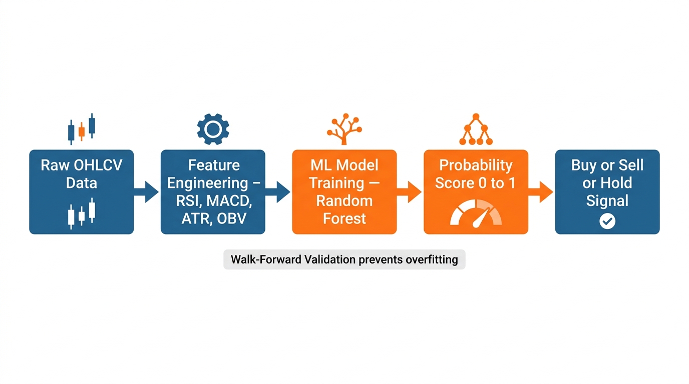
Every rule-based trading strategy contains a hidden assumption: the rules you wrote yesterday will still be valid tomorrow. Moving average crossovers, RSI thresholds, ATR-based stops — these rules are fixed. They were calibrated on historical data, and they will keep firing with exactly the same logic regardless of whether market structure has evolved, volatility has shifted, or correlations have broken down.

Machine learning does something fundamentally different. Instead of encoding fixed rules, it learns the relationship between inputs and outcomes from data. When you feed a machine learning model 50 technical indicators computed from price and volume history and show it thousands of examples of what price did next, it can discover non-linear, multi-dimensional patterns that no human would think to encode as a rule. It can learn that when RSI is above 55 AND ADX is between 22 and 30 AND volume is 1.4× average AND the 20-EMA slope has been positive for six bars, the probability of a 2% gain in the next five days is 68% — not because anyone told it that combination mattered, but because that combination appeared in the training data repeatedly before profitable moves.

This is the genuine promise of AI-powered trading strategies: not the replacement of indicators, but their intelligent combination. The indicators you already know — RSI, MACD, Bollinger Bands, ATR, OBV — become features fed into a model that learns which combinations predict favorable outcomes, and with what confidence.

Feature Engineering: The Real Competitive Advantage

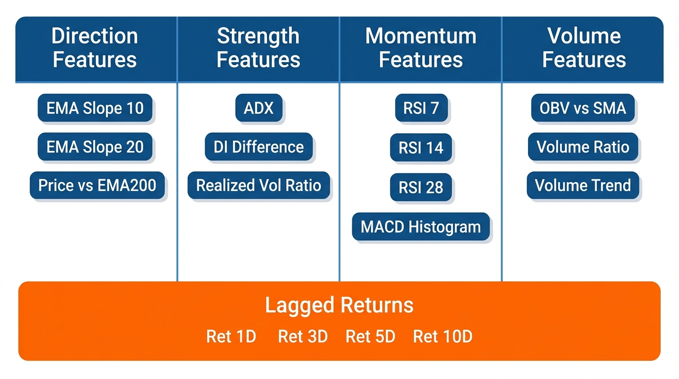
The quality of features determines model performance far more than model choice. A comprehensive feature set includes:

Trend Features: EMA slopes (5, 10, 20, 50-period), MACD line and histogram, ADX value and slope, price relative to EMAs

Momentum Features: RSI (7, 14, 21-period), Stochastic %K and %D, Williams %R, rate of change (ROC)

Volatility Features: ATR, Bollinger Band width and %B, historical volatility (10, 20-period)

Volume Features: OBV and OBV slope, volume ratio vs. 20-day average, volume trend (5-period SMA of volume)

Market Structure Features: Distance to 20-day high/low, number of consecutive higher highs, swing point proximity

1import pandas as pd
2import numpy as np
3import pandas_ta as ta
4
5def engineer_features(df):
6    """Engineer a comprehensive feature set from OHLCV data."""
7    df = df.copy()
8    features = pd.DataFrame(index=df.index)
9
10    # Price-based features
11    features['returns_1d'] = df['close'].pct_change(1)
12    features['returns_5d'] = df['close'].pct_change(5)
13    features['returns_20d'] = df['close'].pct_change(20)
14
15    # EMA distances (normalized)
16    for period in [5, 10, 20, 50, 200]:
17        ema = ta.ema(df['close'], length=period)
18        features[f'ema_{period}_dist'] = (df['close'] - ema) / df['close']
19
20    # RSI
21    for period in [7, 14, 21]:
22        features[f'rsi_{period}'] = ta.rsi(df['close'], length=period)
23
24    # MACD
25    macd = ta.macd(df['close'], fast=12, slow=26, signal=9)
26    features['macd'] = macd['MACD_12_26_9']
27    features['macd_hist'] = macd['MACDh_12_26_9']
28
29    # ADX
30    adx = ta.adx(df['high'], df['low'], df['close'], length=14)
31    features['adx'] = adx['ADX_14']
32
33    # ATR and volatility
34    features['atr'] = ta.atr(df['high'], df['low'], df['close'], length=14)
35    features['atr_pct'] = features['atr'] / df['close']
36
37    # Bollinger Bands
38    bb = ta.bbands(df['close'], length=20, std=2)
39    features['bb_width'] = (bb['BBU_20_2.0'] - bb['BBL_20_2.0']) / bb['BBM_20_2.0']
40    features['bb_pct_b'] = (df['close'] - bb['BBL_20_2.0']) / (bb['BBU_20_2.0'] - bb['BBL_20_2.0'])
41
42    # Volume features
43    features['volume_ratio'] = df['volume'] / df['volume'].rolling(20).mean()
44    features['obv'] = ta.obv(df['close'], df['volume'])
45    features['obv_roc'] = features['obv'].pct_change(5)
46
47    # Target: future N-day return direction
48    features['target'] = (df['close'].shift(-5) / df['close'] - 1 > 0.02).astype(int)
49
50    return features.dropna()

Model Training with Walk-Forward Validation

Walk-forward validation is the gold standard for time series model evaluation. Unlike random train/test splits (which leak future information into training), walk-forward simulates exactly how the model would be deployed in production:

1from sklearn.ensemble import RandomForestClassifier
2from sklearn.metrics import accuracy_score, precision_score
3
4def walk_forward_validation(df, train_window=252, test_window=63):
5    """Walk-forward validation for time series ML strategy."""
6    results = []
7
8    for start in range(0, len(df) - train_window - test_window, test_window):
9        train = df.iloc[start:start + train_window]
10        test = df.iloc[start + train_window:start + train_window + test_window]
11
12        X_train, y_train = train.drop('target', axis=1), train['target']
13        X_test, y_test = test.drop('target', axis=1), test['target']
14
15        model = RandomForestClassifier(
16            n_estimators=200, max_depth=8, min_samples_leaf=50,
17            random_state=42, n_jobs=-1
18        )
19        model.fit(X_train, y_train)
20
21        preds = model.predict(X_test)
22        probs = model.predict_proba(X_test)[:, 1]
23
24        results.append({
25            'period_start': test.index[0],
26            'accuracy': accuracy_score(y_test, preds),
27            'precision': precision_score(y_test, preds),
28            'signal_pct': probs.mean()
29        })
30
31    return pd.DataFrame(results)

A Random Forest with max_depth=8 and min_samples_leaf=50 provides inherent regularization — the depth limit prevents overfitting to noise, and the leaf minimum ensures splits are supported by meaningful sample sizes.

Signal Generation and Position Sizing

The model outputs a probability $p$ that the target return will be positive. This probability becomes a signal strength score:

1def generate_ml_signals(df, model, confidence_threshold=0.60):
2    """Generate trading signals with confidence-based sizing."""
3    X = df.drop('target', axis=1)
4    probs = model.predict_proba(X)[:, 1]
5
6    signals = pd.DataFrame(index=df.index)
7    signals['long_signal'] = probs > confidence_threshold
8    signals['confidence'] = probs
9    signals['position_multiplier'] = np.where(
10        probs > confidence_threshold,
11        (probs - confidence_threshold) / (1 - confidence_threshold),
12        0
13    )
14
15    return signals

Positions are sized proportionally to model confidence — higher probability predictions receive larger allocations, while borderline signals receive minimal exposure. This transforms a binary classifier into a continuous capital allocation system.

Interpreting the Model with SHAP

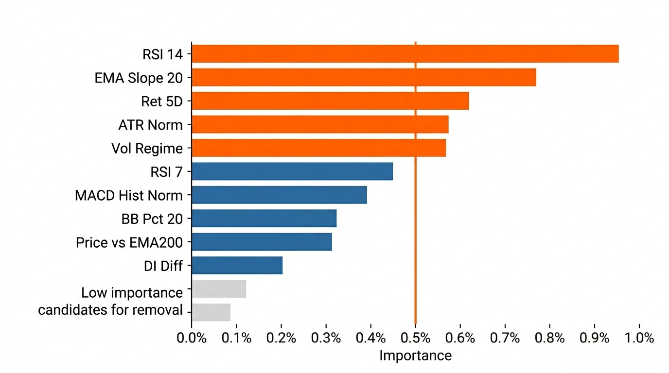
Black-box models are dangerous in trading. SHAP (SHapley Additive exPlanations) values decompose each prediction into feature contributions, telling you exactly which indicators drove the decision:

1import shap
2
3explainer = shap.TreeExplainer(model)
4shap_values = explainer.shap_values(X_test.iloc[:100])
5
6# Plot feature importance
7shap.summary_plot(shap_values[1], X_test.iloc[:100],
8                  feature_names=X_test.columns, show=False)

This interpretability is critical for debugging: if the model suddenly changes behavior in live trading, SHAP analysis reveals which features drove the shift and whether it's a legitimate regime change or a data problem.

The Limitations (And Why They Matter)

1. Regime change is the enemy — models trained in low-volatility bull markets will fail in high-volatility bear markets unless retrained
2. Overfitting is easier than it looks — 50 features × 200 trees = many degrees of freedom; walk-forward validation is your only defense
3. ML amplifies data quality issues — survivorship bias, lookahead leakage, and poor data hygiene are magnified
4. Interpretability is not optional — if you cannot explain why your model is long, you should not trust its recommendation

Key Takeaways

• Feature engineering is the competitive advantage — the quality and breadth of indicator features matter more than model selection
• Walk-forward validation is mandatory — random train/test splits are invalid for time series; walk-forward simulates deployment
• Confidence-based position sizing transforms ML from a binary signal into a continuous capital allocation framework
• SHAP provides interpretability — understanding why the model predicts what it does is essential for trust and debugging
• Regime change is the primary risk — a model is only valid in conditions similar to its training data; monitor for drift continuously

Conclusion

Machine learning does not replace technical indicators — it amplifies them. Where a human trader might combine three or four indicators into a discretionary decision, an ML model can systematically evaluate fifty indicators, learn their non-linear interactions, and output a calibrated probability. That probability becomes the foundation of a systematic trading strategy that adapts to data rather than imposing fixed thresholds.

Your next step: build the feature engineering pipeline, train a Random Forest on the first 70% of your data, validate on the remaining 30% using walk-forward windows, and compare the filtered signals against your existing rule-based strategies. The goal is not to replace what works — it's to make what works work better.