AI Models That Predict Crypto Markets: What Actually Works and Why

Introduction: The Model That Saw the Crash Coming

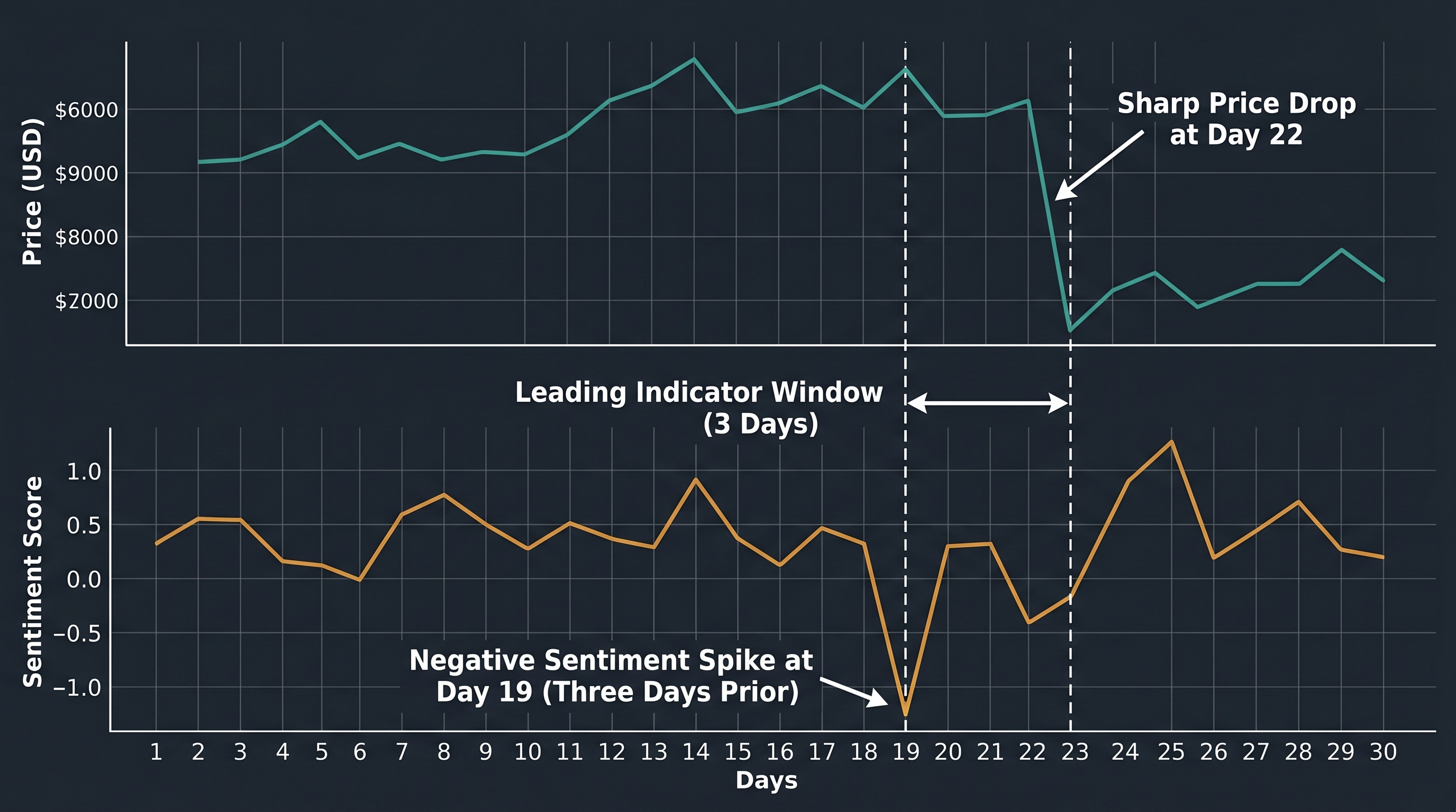
In late 2022, as FTX collapsed and sent shockwaves through the entire crypto market, most traders were caught completely off guard. But a small group of quantitative funds had already reduced their exposure days earlier — not because of insider information, but because their sentiment analysis models had detected an unusual spike in negative language across crypto forums and social media that historically preceded sharp drawdowns.

No chart pattern flagged it. No technical indicator blinked red. An AI model reading text did.

This is the reality of AI-powered crypto trading in 2024: the edge is no longer just in price data. It is in processing information faster, from more sources, with more consistency than any human team can manage. And the traders who understand which AI models actually work — and more importantly, why they work — are the ones building strategies that compound quietly while everyone else chases the next narrative.

In this post, you will learn the core AI architectures being applied to crypto market prediction right now, how each one processes market data differently, where each genuinely excels and where each quietly fails, and how to implement a working sequence prediction model in Python. By the end, you will not only understand these models conceptually — you will know how to start using them.

If you leave now, you will keep trading with yesterday's tools. Stay, and you will finish with tomorrow's.

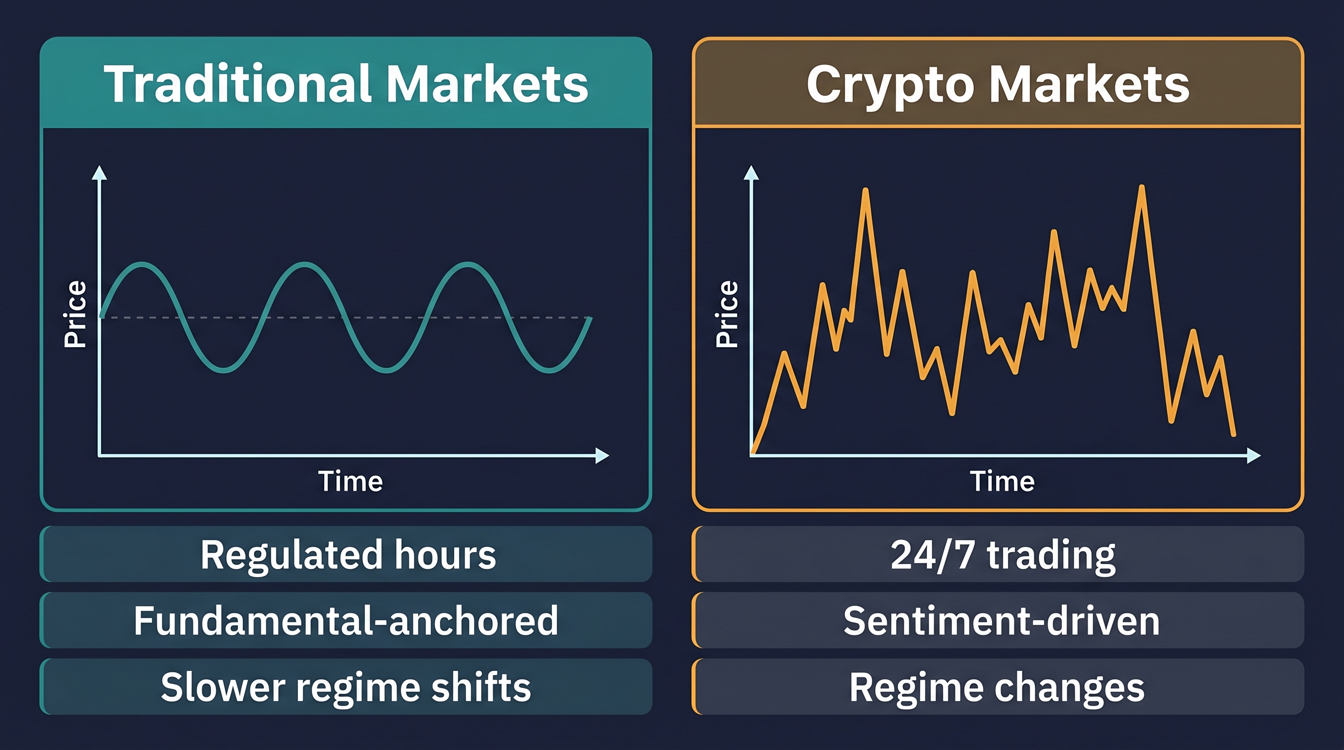
Why Crypto Is Both a Dream and a Nightmare for AI Models

Before evaluating specific models, it is worth confronting an uncomfortable truth: crypto markets are among the most difficult environments on earth for prediction models. Understanding why is not discouraging — it is essential. It tells you exactly what to demand from any model you build or evaluate.

Crypto markets operate 24 hours a day, 365 days a year, across hundreds of fragmented exchanges simultaneously. They are driven by a uniquely volatile cocktail of retail speculation, institutional flows, regulatory headlines, Twitter sentiment, macroeconomic data, and on-chain activity. The signal-to-noise ratio is punishingly low.

And yet — and this is the key insight — short-horizon inefficiencies persist. Not because crypto is irrational, but because the sheer volume and diversity of information moving through the market creates temporary imbalances that models can exploit before human traders process and act on the same information.

The models that succeed do not predict the future with certainty. They shift probabilities slightly but consistently in their favor, and then position sizing and risk management do the rest of the work.

The Core AI Models Applied to Crypto Price Prediction

Not all AI models are built the same, and not all of them belong in a trading system. Here is an honest, technical breakdown of the models that have demonstrated genuine utility in crypto market prediction — along with what each one actually does under the hood.

LSTM: The Model That Remembers

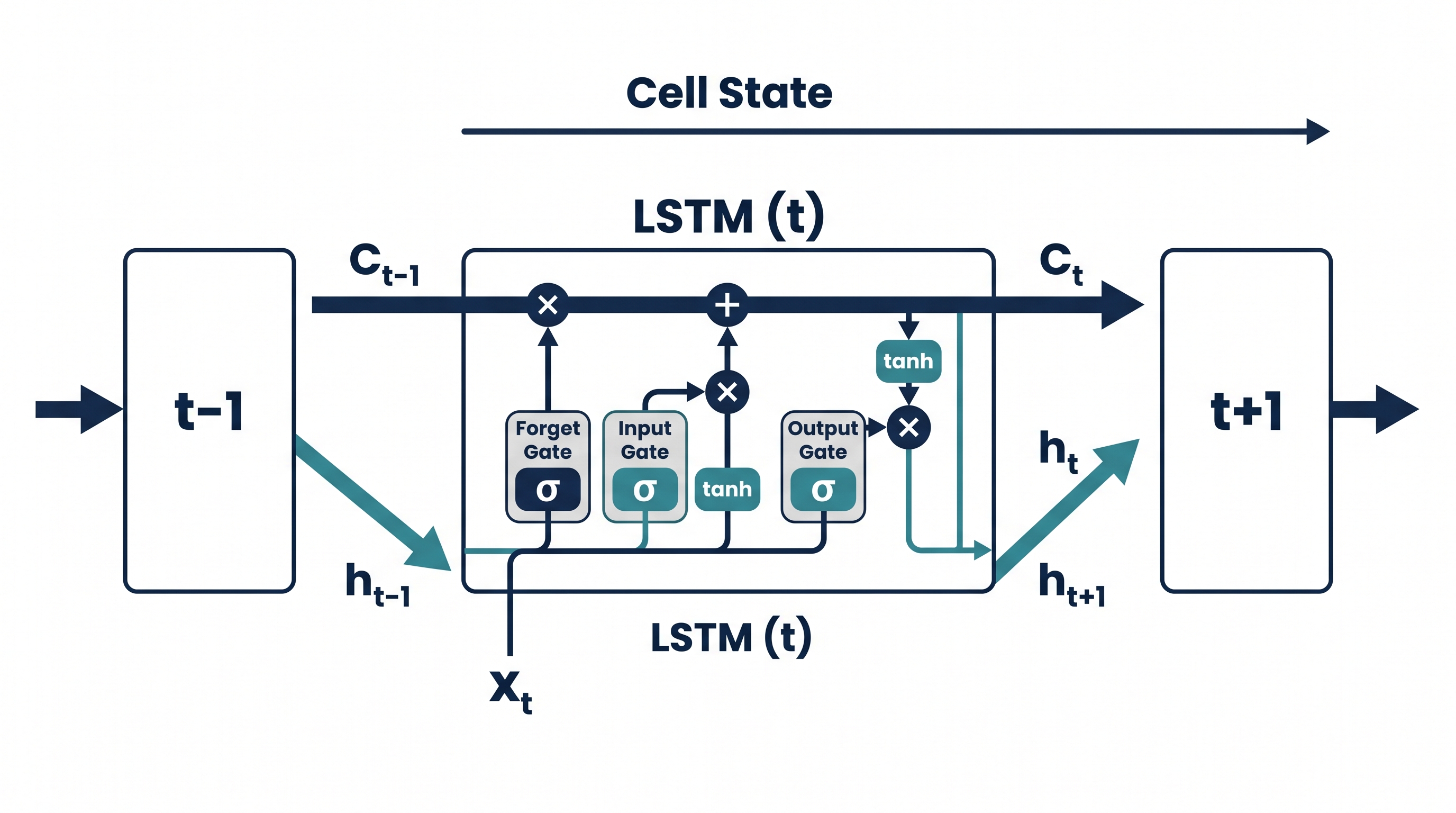
Long Short-Term Memory networks, or LSTMs, were for several years the dominant architecture for financial time-series prediction, and they remain widely used today. To understand why, you first need to understand the problem they were designed to solve.

Standard neural networks process each input independently. They have no memory of what came before. For price prediction, this is a critical limitation — the price of Bitcoin at 3:00 PM is deeply related to what happened at 2:00 PM, 1:00 PM, and the three days prior. Sequence matters.

LSTMs solve this by maintaining a hidden state — a kind of internal memory — that persists across time steps. At each step, the network decides what new information to write into memory, what old information to erase, and what to output based on the current memory state. These decisions are governed by three learned gates:

The Forget Gate — decides what fraction of the previous memory to retain:

The Input Gate — decides what new information to add to memory:

The Output Gate — decides what the network outputs at this step:

Where $h_{t}$ is the hidden state, $x_{t}$ is the current input, $C_{t}$ is the cell state (memory), and $W$ and $b$ are learned weights and biases. $\sigma$ is the sigmoid activation function, which squashes values between 0 and 1.

In plain English: the LSTM learns which parts of market history are worth remembering and which are noise. That learned selectivity is precisely what makes it useful for financial sequences.

Transformer Models: Attention Without Sequence Bottlenecks

LSTMs process sequences step by step, which creates a bottleneck: information from early in the sequence must be compressed and passed forward through every subsequent step. For very long sequences, this compression degrades signal quality.

Transformers — the architecture behind GPT and BERT — solve this with a mechanism called self-attention, which allows the model to directly compare every time step in a sequence to every other time step simultaneously, without the sequential bottleneck.

The attention score between any two time steps is computed as:

Where $Q$ (queries), $K$ (keys), and $V$ (values) are learned linear projections of the input, and $d_{k}$ is the dimension of the key vectors. The $\sqrt{d_{k}}$ scaling factor prevents the dot products from growing too large in magnitude.

In trading terms, this means a transformer applied to 90 days of price data can directly learn that "conditions on day 3 are highly relevant to predicting day 87" — without having to carry that information forward through 84 intermediate steps the way an LSTM would.

Recent research has shown transformer-based models outperforming LSTMs on crypto prediction tasks, particularly when working with longer lookback windows and multiple asset inputs simultaneously.

Gradient Boosting: The Surprisingly Competitive Baseline

If LSTMs and transformers are the flashy architectures, XGBoost and LightGBM are the quietly dominant workhorses of production quantitative trading. Multiple industry surveys of professional quant researchers consistently find gradient boosted trees outperforming deep learning on tabular financial data — and crypto price prediction with engineered features is fundamentally a tabular problem.

Gradient boosting builds an ensemble of decision trees sequentially, where each new tree is trained to correct the prediction errors of all previous trees. The final prediction is:

Where $h_{m}(x)$ is the $m$-th tree, $M$ is the total number of trees, and $\eta$ is the learning rate controlling how much each tree contributes. The learning rate acts as a regularization mechanism — smaller values require more trees but generally generalize better.

The reason gradient boosting often beats deep learning on financial tabular data comes down to data efficiency: LSTMs and transformers require substantial data to learn well. Gradient boosting achieves strong performance with far fewer samples, which matters enormously in crypto where certain market regimes have limited historical examples.

Sentiment Models: The Hidden Information Layer

The most underappreciated category of AI model in crypto trading is natural language processing (NLP) applied to sentiment analysis. While price models look at what has happened, sentiment models attempt to measure what the crowd is thinking — which frequently leads price moves rather than lagging them.

Modern sentiment models for crypto typically use pre-trained transformer architectures (such as FinBERT, a version of BERT fine-tuned on financial text) to classify social media posts, news headlines, and forum discussions as positive, negative, or neutral — and then aggregate these classifications into a quantitative sentiment score.

The sentiment score at time $t$ can be computed as:

Where $s_{i}$ is the sentiment score of the $i$-th document (typically ranging from -1 to +1), $w_{i}$ is a recency or source-credibility weight, and $N$ is the total number of documents in the aggregation window.

Spikes in negative sentiment — particularly when they diverge from price action — have historically been leading indicators of drawdowns in Bitcoin and major altcoins.

Building an LSTM Price Prediction Model in Python

Theory becomes strategy only when it runs in code. Here is a step-by-step implementation of an LSTM that predicts Bitcoin's next-day closing price direction using Keras and TensorFlow.

Step 1 — Data Preparation and Feature Scaling

1import numpy as np
2import pandas as pd

from sklearn.preprocessing import MinMaxScaler

from tensorflow.keras.models import Sequential

from tensorflow.keras.layers import LSTM, Dense, Dropout

from tensorflow.keras.callbacks import EarlyStopping

1# Load OHLCV data
2df = pd.read_csv('btc_daily.csv', parse_dates=['timestamp'], index_col='timestamp')
3df = df[['close', 'volume']].dropna()
4
5# Scale features to [0, 1] range — critical for LSTM stability
6scaler = MinMaxScaler()
7scaled = scaler.fit_transform(df)

Scaling is not optional with LSTMs. The sigmoid and tanh activation functions used inside LSTM gates saturate at extreme values, which kills gradient flow and prevents the network from learning. MinMaxScaler compresses all values into the range [0, 1], keeping activations in the sensitive, informative region of those functions.

Step 2 — Create Sequence Windows

1def create_sequences(data, lookback=30):

X, y = [], []

for i in range(lookback, len(data)):

1X.append(data[i - lookback:i])   # Past 30 days as input
2y.append(data[i, 0])             # Next day's close as target
3return np.array(X), np.array(y)
4
5lookback = 30

X, y = create_sequences(scaled, lookback)

1# Chronological train/test split — never shuffle time-series data
2split = int(len(X) * 0.8)

X_train, X_test = X[:split], X[split:]

y_train, y_test = y[:split], y[split:]

1print(f"Training samples: {len(X_train)}, Test samples: {len(X_test)}")

Each input sample $X_{i}$ is a window of 30 consecutive days, and the corresponding label $y_{i}$ is the closing price on day 31. Sliding this window across the entire dataset generates all training samples. The 80/20 split is strictly chronological — future data never contaminates training.

Step 3 — Build and Train the LSTM

model = Sequential([

LSTM(64, return_sequences=True, input_shape=(lookback, X.shape[2])),

Dropout(0.2),

LSTM(32, return_sequences=False),

Dropout(0.2),

Dense(1)

])

model.compile(optimizer='adam', loss='mean_squared_error')

early_stop = EarlyStopping(monitor='val_loss', patience=10, restore_best_weights=True)

history = model.fit(

X_train, y_train,

epochs=100,

batch_size=32,

validation_split=0.1,

callbacks=[early_stop],

verbose=1

)

A few design choices worth understanding here. The two stacked LSTM layers allow the network to learn features at different levels of abstraction — the first layer captures short-term patterns, the second synthesizes those into higher-level sequence structure. Dropout layers randomly deactivate 20% of neurons during training, which forces the network to learn redundant representations and dramatically reduces overfitting. Early stopping halts training when validation loss stops improving, preventing the model from memorizing the training data.

Step 4 — Evaluate and Inverse Transform Predictions

1# Generate predictions on test set
2predictions_scaled = model.predict(X_test)
3
4# Reconstruct full-dimensional array for inverse transform
5pred_full = np.zeros((len(predictions_scaled), scaled.shape[1]))

pred_full[:, 0] = predictions_scaled[:, 0]

1actual_full = np.zeros((len(y_test), scaled.shape[1]))

actual_full[:, 0] = y_test

1# Inverse transform to get real price values
2predictions = scaler.inverse_transform(pred_full)[:, 0]
3actuals = scaler.inverse_transform(actual_full)[:, 0]
4
5# Root Mean Squared Error
6rmse = np.sqrt(np.mean((predictions - actuals) ** 2))
7print(f"RMSE: ${rmse:,.2f}")

The inverse transform step is critical: your model outputs scaled values between 0 and 1. To interpret them as actual prices, you must reverse the scaling transformation using the same scaler fitted on the training data.

The Root Mean Squared Error (RMSE) provides a baseline quality metric:

Where $\hat{y}*{i}$ is the predicted price and $y*{i}$ is the actual price. A lower RMSE indicates predictions are closer to reality, though RMSE alone is insufficient for evaluating a trading strategy — what ultimately matters is risk-adjusted return, not prediction accuracy in dollar terms.

Honest Limitations: What These Models Cannot Do

Intellectual honesty about model limitations is what separates serious practitioners from people who lose money on backtests that never worked to begin with.

LSTMs suffer from vanishing gradients on very long sequences. Despite their gating mechanism, LSTMs still struggle to reliably carry information across sequences longer than a few hundred time steps. For daily crypto data, this means anything beyond roughly six months of history becomes increasingly unreliable as direct input.

Transformers are data-hungry. The self-attention mechanism requires substantial data to learn meaningful relationships. With crypto's relatively short historical record compared to equities, transformers risk overfitting unless carefully regularized and supplemented with data augmentation techniques.

All models are regime-blind by default. A model trained in a bull market learns bull market patterns. When the regime shifts to a bear market, those patterns may invert entirely. Without explicit regime detection — either through clustering methods or regime-switching models — your AI can confidently predict the wrong direction.

Sentiment models degrade rapidly. The language of crypto communities evolves constantly. Slang, memes, and irony make NLP classification significantly harder than in traditional financial text. A sentiment model trained in 2021 may interpret 2024 crypto Twitter very differently than intended.

The appropriate response to these limitations is not to abandon AI models — it is to build systems that monitor model performance in real time and trigger retraining or position reduction when performance degrades beyond acceptable thresholds.

Key Takeaways

• LSTMs learn sequential dependencies in price data through learned memory gates, making them suitable for capturing short-to-medium-term temporal patterns in crypto markets.
• Transformers use self-attention to compare all time steps in a sequence simultaneously, avoiding the sequential bottleneck of LSTMs and outperforming them on longer lookback windows.
• Gradient boosted models frequently outperform deep learning on tabular crypto data with engineered features, particularly when training data is limited.
• Sentiment AI models using NLP on social and news data can act as leading indicators, detecting crowd psychology shifts before they fully manifest in price.
• No AI model eliminates prediction uncertainty. Models shift probabilities incrementally — position sizing and risk management determine whether those incremental edges translate into actual profit.
• Regime awareness, periodic retraining, and real-time performance monitoring are non-negotiable requirements for deploying AI models in live crypto trading.

Conclusion: The Edge Is in the Process, Not the Model

After reading this far, you now understand something that most retail crypto traders will never take the time to learn: the model itself is not the edge. The edge is in the process — the disciplined feature engineering, the honest evaluation methodology, the regime awareness, the willingness to retrain when markets change, and the risk management that protects capital while the model learns.

The traders who will dominate the next cycle of crypto markets are not the ones who find the "magic" model. They are the ones who build robust pipelines that process information systematically, evaluate themselves honestly, and adapt continuously.

You have the conceptual foundation now. The LSTM code in this post runs on any daily OHLCV dataset you can download from Binance, Kraken, or CoinGecko. Start there. Run it. Break it intentionally — remove dropout, expand the feature set, shorten the training window — and watch what happens to your validation loss. Each experiment teaches you something a blog post cannot.

The market does not reward the most confident trader. It rewards the most prepared one.

Explore the rest of this series for deep dives into backtesting AI-generated signals, combining sentiment with price models into multi-modal prediction systems, and building the live execution infrastructure that turns a working model into a running strategy. Each layer compounds on the last.

Your preparation starts now.