ADX Strategy for Finding Strong Crypto Market Trends in Algorithmic Trading

Introduction: Most Crypto Traders Are Trading the Wrong Market Condition

Here is a counterintuitive truth that professional systematic traders understand and most retail crypto traders never fully internalize: the single biggest determinant of whether a trend-following strategy makes money is not the entry signal. It is whether the market is actually trending in the first place.

A moving average crossover applied to a trending Bitcoin market can look like genius. Applied to the same market three months later in a sideways chop, the same strategy generates an unbroken sequence of losses. The indicator has not changed. The signal logic has not changed. The market regime has changed — and if you are not measuring it, you are trading blind.

This is precisely the problem the Average Directional Index, or ADX, was designed to solve. ADX does not tell you which direction the market is moving. It tells you whether the market is moving at all — with enough directional conviction to justify a trend-following entry. It separates the high-probability trend environments from the choppy, mean-reverting conditions where trend signals are nothing but noise.

In this post, you will learn how ADX is constructed mathematically from its component parts, implement it in Python from scratch, understand how to read ADX values in the context of crypto volatility, build a complete ADX-based trend-following strategy for crypto markets, and extend that strategy with a multi-timeframe confirmation filter that dramatically improves signal quality. This is the systematic framework for finding the strong crypto trends that produce outsized returns — and avoiding the conditions that destroy trend strategies.

Section 1: The ADX Concept — Measuring Trend Strength Without Direction Bias

What Makes ADX Fundamentally Different from Every Other Trend Indicator

Most trend indicators — moving averages, MACD, Supertrend — tell you which direction the market is trending. ADX tells you something different and in many ways more valuable: how strongly the market is trending, regardless of direction. This is not a subtle distinction. It is the difference between knowing you are in a trend and knowing whether you are in a market worth trading at all.

ADX is derived from two directional movement indicators — the Positive Directional Indicator and the Negative Directional Indicator, denoted $+DI$ and $-DI$ — which together measure the relative strength of upward and downward price movement. ADX itself is then derived from the relationship between these two indicators, producing a single oscillator that rises when either the uptrend or the downtrend is strengthening and falls when neither has conviction.

This architecture means ADX is immune to the directional bias that afflicts most trend indicators. A market that is trending sharply downward will produce a high ADX reading, just as a sharply upward-trending market will. What produces a low ADX reading is a market moving sideways — oscillating without sustained directional conviction — precisely the condition where trend-following entries are most dangerous.

Section 2: ADX Construction — The Mathematics from First Principles

You Cannot Trust an Indicator You Cannot Build Yourself

ADX is computed through a sequence of steps, each building on the previous one. Understanding this construction is not just academic — it reveals exactly what ADX is sensitive to and how to interpret its readings correctly.

Step 1: Directional Movement

At each bar, the upward and downward directional movement is computed by comparing the current bar's high and low to the previous bar's high and low:

In plain English: $+DM$ captures how much today's high exceeded yesterday's high, but only when that upward expansion was larger than any downward expansion and was positive. $-DM$ captures how much today's low fell below yesterday's low under equivalent conditions. The two cannot both be non-zero on the same bar — only the dominant directional move is counted.

Step 2: Smoothed Directional Movement and ATR

Both directional movement values and the True Range are smoothed using Wilder's exponential smoothing over $n$ periods (typically 14):

The same Wilder smoothing is applied to the True Range to produce ATR.

Step 3: The Directional Indicators

The smoothed directional movements are normalized by ATR to produce the $+DI$ and $-DI$ values, expressed as percentages:

When $+DI$ is above $-DI$, upward movement is dominant — a bullish condition. When $-DI$ is above $+DI$, downward movement is dominant — a bearish condition. The separation between the two lines is a rough indicator of directional conviction.

Step 4: The Directional Index and ADX

The Directional Index (DX) measures the relative difference between $+DI$ and $-DI$:

ADX is then the Wilder-smoothed average of DX over $n$ periods:

The result is an oscillator between 0 and 100. Values above 25 indicate a trending market; values above 50 indicate a strongly trending market. Values below 20 indicate a ranging or trendless market where trend-following strategies should typically be inactive.

Section 3: Implementing ADX in Python

From Mathematics to Code — A Clean, Reusable Implementation

The following Python implementation builds ADX step by step, matching Wilder's original methodology:

1import numpy as np
2import pandas as pd
3
4def wilder_smooth(series, period):

"""

Apply Wilder's exponential smoothing to a series.

Parameters:

1series: pd.Series of values to smooth

period: int, smoothing period

Returns:

1pd.Series of smoothed values

"""

1series = pd.Series(series).reset_index(drop=True)
2smoothed = pd.Series(index=series.index, dtype=float)
3
4# Seed with simple sum of first `period` values
5smoothed.iloc[period - 1] = series.iloc[:period].sum()

for i in range(period, len(series)):

smoothed.iloc[i] = smoothed.iloc[i - 1] - (smoothed.iloc[i - 1] / period) + series.iloc[i]

1return smoothed
2
3def compute_adx(high, low, close, period=14):

"""

Compute ADX, +DI, and -DI from OHLC data.

Parameters:

1high: pd.Series of bar high prices
2low: pd.Series of bar low prices
3close: pd.Series of bar close prices

period: int, ADX smoothing period (default 14)

Returns:

1pd.DataFrame with columns 'adx', 'plus_di', 'minus_di'

"""

1high = pd.Series(high).reset_index(drop=True)
2low = pd.Series(low).reset_index(drop=True)
3close = pd.Series(close).reset_index(drop=True)
4
5# True Range
6prev_close = close.shift(1)
7tr = pd.concat([

high - low,

(high - prev_close).abs(),

(low - prev_close).abs()

1], axis=1).max(axis=1)
2
3# Directional Movement
4up_move = high - high.shift(1)
5down_move = low.shift(1) - low
6
7plus_dm = np.where((up_move > down_move) & (up_move > 0), up_move, 0.0)
8minus_dm = np.where((down_move > up_move) & (down_move > 0), down_move, 0.0)
9
10plus_dm = pd.Series(plus_dm, index=high.index)
11minus_dm = pd.Series(minus_dm, index=high.index)
12
13# Wilder smoothing
14smoothed_tr = wilder_smooth(tr, period)
15smoothed_plus_dm = wilder_smooth(plus_dm, period)
16smoothed_minus_dm = wilder_smooth(minus_dm, period)
17
18# Directional Indicators

plus_di = (smoothed_plus_dm / smoothed_tr) * 100

minus_di = (smoothed_minus_dm / smoothed_tr) * 100

1# DX and ADX

dx = (abs(plus_di - minus_di) / (plus_di + minus_di)) * 100

1dx = dx.replace([np.inf, -np.inf], np.nan).fillna(0)
2
3adx = pd.Series(index=dx.index, dtype=float)
4adx.iloc[period * 2 - 2] = dx.iloc[period - 1: period * 2 - 1].mean()

for i in range(period * 2 - 1, len(dx)):

adx.iloc[i] = (adx.iloc[i - 1] * (period - 1) + dx.iloc[i]) / period

1return pd.DataFrame({
2'adx': adx,
3'plus_di': plus_di,
4'minus_di': minus_di

})

After computing ADX, validate it against a reference platform such as TradingView or a financial data library like pandas_ta. Close agreement after the warmup period of approximately $2 \times n$ bars confirms a correct implementation.

Section 4: Reading ADX Values in Crypto Context

Why Crypto Requires Different ADX Thresholds Than Equity Markets

The standard ADX interpretation — above 25 is trending, below 20 is ranging — was developed in the context of equity and futures markets. Crypto markets have substantially different volatility characteristics, which affects how ADX values should be interpreted.

Because crypto assets frequently experience rapid regime changes — transitioning from extremely strong trends to violent chop in days rather than weeks — ADX in crypto tends to be more volatile as an indicator itself, rising and falling more quickly than in equity markets. This means two practical adjustments are worth considering.

First, the trending threshold may need to be higher in crypto. In equity markets, an ADX of 25 reliably indicates a meaningful trend. In some crypto markets, particularly altcoins with erratic volatility, an ADX threshold of 30 or even 35 produces better signal quality by filtering out the more marginal trending conditions that are common in crypto and which tend to generate more false signals.

Second, ADX rate of change matters as much as its level. An ADX reading of 30 that has been declining for five bars indicates a trend that is losing momentum — a different risk profile from an ADX of 30 that has been rising for five bars, indicating an accelerating trend. Monitoring the slope of ADX, not just its level, adds an important dimension to the signal:

1def adx_slope(adx_series, lookback=3):

"""

Compute the slope of the ADX line over a rolling window.

Positive slope = trend strengthening; negative slope = trend weakening.

Parameters:

1adx_series: pd.Series of ADX values

lookback: int, number of bars for slope calculation

Returns:

1pd.Series of ADX slope values

"""

1return adx_series.diff(lookback)

A slope above zero means ADX is rising — trend is strengthening. A slope below zero means ADX is falling — trend may be exhausting. Requiring both a minimum ADX level and a positive slope before entering a trend trade ensures you are joining a trend that is developing, not one that has already peaked.

Section 5: Building a Complete ADX Trend-Following Strategy for Crypto

Combining ADX with Directional Signals for a Full Trading System

ADX alone does not tell you which direction to trade — it only tells you whether trading is worthwhile at all. The complete strategy combines ADX as a regime filter with $+DI$ and $-DI$ crossovers (or another directional signal) to produce directional entries only in confirmed trending conditions.

The entry rules for the core ADX crypto trend strategy are:

Long entry: ADX above threshold AND ADX slope positive AND $+DI$ crosses above $-DI$

Short entry: ADX above threshold AND ADX slope positive AND $-DI$ crosses above $+DI$

Exit: ADX falls below the threshold OR the directional crossover reverses

1def adx_trend_signals(high, low, close,
2adx_period=14,
3adx_threshold=25,
4slope_lookback=3,
5require_positive_slope=True):

"""

Generate long/short entry signals from ADX trend strategy.

Parameters:

1high, low, close: pd.Series of OHLC data

adx_period: int, ADX period

adx_threshold: float, minimum ADX for trending regime (25 for equities, 30 for crypto)

slope_lookback: int, bars for ADX slope computation

require_positive_slope: bool, require rising ADX for entry

Returns:

1pd.DataFrame with signal columns

"""

1high = pd.Series(high).reset_index(drop=True)
2low = pd.Series(low).reset_index(drop=True)
3close = pd.Series(close).reset_index(drop=True)
4
5adx_df = compute_adx(high, low, close, adx_period)
6adx = adx_df['adx']
7plus_di = adx_df['plus_di']
8minus_di = adx_df['minus_di']
9slope = adx_slope(adx, slope_lookback)
10
11# Regime filter: ADX above threshold
12trending = adx >= adx_threshold

if require_positive_slope:

trending = trending & (slope > 0)

1# Directional crossovers
2plus_di_cross_above = (plus_di > minus_di) & (plus_di.shift(1) <= minus_di.shift(1))
3minus_di_cross_above = (minus_di > plus_di) & (minus_di.shift(1) <= plus_di.shift(1))
4
5long_entry = trending & plus_di_cross_above
6short_entry = trending & minus_di_cross_above
7
8# Exit when ADX drops below threshold
9exit_signal = adx < (adx_threshold - 5)  # 5-point buffer to prevent whipsaw exits
10
11return pd.DataFrame({
12'adx': adx,
13'plus_di': plus_di,
14'minus_di': minus_di,
15'slope': slope,
16'trending': trending,
17'long_entry': long_entry,
18'short_entry': short_entry,
19'exit_signal': exit_signal

})

The five-point buffer on the exit condition deserves explanation. If the ADX threshold for entry is 25 and the exit triggers immediately when ADX drops below 25, every brief dip of ADX to 24 generates a trade exit followed by a potential re-entry — unnecessary churn that increases transaction costs and can create a sequence of false stops. Using a lower exit threshold of 20 (or $\text{threshold} - 5$) prevents this by requiring a more definitive drop in trend strength before exiting.

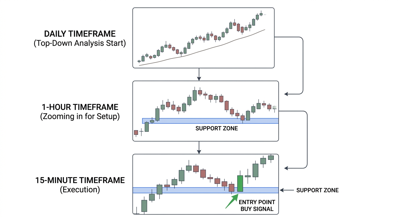
Section 6: Multi-Timeframe ADX Confirmation for Higher-Quality Crypto Signals

The Single Most Effective Enhancement to Any ADX-Based Strategy

A trend identified on a single timeframe can be a genuine multi-week directional move or a transient spike that quickly reverses. Multi-timeframe analysis addresses this ambiguity by requiring the same trending condition to be confirmed on a higher timeframe before acting on the lower-timeframe signal.

The principle is straightforward: if the daily ADX confirms a trend and the 4-hour ADX also confirms a trend in the same direction, that alignment across timeframes provides substantially stronger evidence of a genuine trending market than either timeframe alone.

1def multi_timeframe_adx_filter(
2htf_high, htf_low, htf_close,   # Higher timeframe OHLC
3ltf_signals_df,                  # Lower timeframe signals from adx_trend_signals()
4htf_adx_period=14,
5htf_adx_threshold=25,
6htf_index_map=None               # Optional: mapping from LTF index to HTF index

):

"""

Apply higher-timeframe ADX confirmation to lower-timeframe signals.

Only allows LTF signals through when HTF is also in a trending regime.

Parameters:

1htf_high, htf_low, htf_close: pd.Series of higher timeframe OHLC
2ltf_signals_df: pd.DataFrame from adx_trend_signals() on lower timeframe

htf_adx_period: int, ADX period for higher timeframe

htf_adx_threshold: float, minimum ADX on higher timeframe

1htf_index_map: optional pd.Series mapping LTF bar index to HTF bar index

Returns:

1pd.DataFrame: filtered signals with HTF confirmation column added

"""

htf_adx_df = compute_adx(htf_high, htf_low, htf_close, htf_adx_period)

1htf_trending = htf_adx_df['adx'] >= htf_adx_threshold
2htf_direction = (htf_adx_df['plus_di'] > htf_adx_df['minus_di']).map(

{True: 1, False: -1}

)

1signals = ltf_signals_df.copy()
2
3# For simplicity: apply HTF filter by reindexing to match LTF length
4# In practice, use proper bar alignment based on timestamps

if htf_index_map is not None:

htf_trend_aligned = htf_trending.reindex(htf_index_map).values

htf_dir_aligned = htf_direction.reindex(htf_index_map).values

else:

1# Simple approach: forward-fill HTF values to LTF length
2repeat_factor = max(1, len(signals) // len(htf_trending))
3htf_trend_aligned = np.repeat(htf_trending.values, repeat_factor)[:len(signals)]
4htf_dir_aligned = np.repeat(htf_direction.values, repeat_factor)[:len(signals)]
5
6htf_trend_series = pd.Series(htf_trend_aligned, index=signals.index)
7htf_dir_series = pd.Series(htf_dir_aligned, index=signals.index)
8
9# Only pass long entries when HTF is trending bullish

signals['long_entry'] = (

signals['long_entry'] &

htf_trend_series &

(htf_dir_series == 1)

)

1# Only pass short entries when HTF is trending bearish

signals['short_entry'] = (

signals['short_entry'] &

htf_trend_series &

(htf_dir_series == -1)

)

signals['htf_trending'] = htf_trend_series

signals['htf_direction'] = htf_dir_series

1return signals

In practice, timeframe alignment requires proper timestamp-based bar mapping — matching each lower-timeframe bar to its corresponding higher-timeframe bar. The simplified approach above is suitable for prototyping and understanding the logic; production implementations should use timestamp indices to ensure correct alignment.

Section 7: ADX Parameter Calibration for Crypto Assets

Crypto Trends Move Fast — Your ADX Parameters Should Reflect That

ADX with its default period of 14 was designed for daily equity charts. For crypto assets — which trade 24/7, exhibit significantly higher volatility, and can complete full trend cycles in days rather than weeks — a shorter period often produces more responsive and actionable readings.

A systematic approach to period selection compares the strategy's Sharpe ratio and profit factor across a range of period and threshold combinations:

1def adx_parameter_search(high, low, close,
2periods=None, thresholds=None):

"""

Grid search to find optimal ADX period and threshold for a crypto asset.

Parameters:

1high, low, close: pd.Series of OHLC data

periods: list of int ADX periods to test

thresholds: list of float ADX threshold values to test

Returns:

1pd.DataFrame of results sorted by Sharpe ratio

"""

if periods is None:

periods = [7, 10, 14, 20]

if thresholds is None:

thresholds = [20, 25, 30, 35]

1close = pd.Series(close).reset_index(drop=True)

results = []

for period in periods:

for threshold in thresholds:

try:

sigs = adx_trend_signals(

high, low, close,

adx_period=period,

adx_threshold=threshold,

require_positive_slope=True

)

1# Simple long-only returns: in market when long_entry is active
2direction = pd.Series(0, index=close.index)
3in_trade = False

for i in range(len(sigs)):

if sigs['long_entry'].iloc[i]:

in_trade = True

if sigs['exit_signal'].iloc[i]:

in_trade = False

direction.iloc[i] = 1 if in_trade else 0

1strategy_returns = direction.shift(1) * close.pct_change()
2strategy_returns = strategy_returns.dropna()
3
4if strategy_returns.std() == 0 or len(strategy_returns) < 50:

continue

1sharpe = (strategy_returns.mean() / strategy_returns.std()) * np.sqrt(365)
2n_trades = sigs['long_entry'].sum()

results.append({

"period": period,

"threshold": threshold,

"sharpe": round(sharpe, 3),

"n_trades": int(n_trades)

})

except Exception:

continue

1return pd.DataFrame(results).sort_values("sharpe", ascending=False)

Always validate optimized parameters on out-of-sample data. Split your full history into a training set (first 70%) and a test set (last 30%). Parameters that perform well on both are far more likely to reflect genuine market structure than parameters optimized on the full dataset.

For Bitcoin and Ethereum on daily charts, periods of 10 to 14 with thresholds of 25 to 30 typically produce robust results. For smaller altcoins on shorter timeframes (4-hour or 1-hour), periods of 7 to 10 with higher thresholds of 30 to 35 are often better calibrated to the more erratic trend behavior of those assets.

Key Takeaways

• ADX measures trend strength without direction bias. A high ADX indicates a strong trend regardless of whether it is bullish or bearish — making it one of the most valuable regime filters available for trend-following strategies.
• The standard ADX threshold of 25 was developed for equity markets. Crypto assets often benefit from higher thresholds of 30 to 35 due to their more volatile and erratic price behavior, which produces more marginal trending conditions that generate false signals.
• ADX slope (rate of change) adds critical information beyond the absolute ADX level. Requiring a positive ADX slope filters for trends that are developing and strengthening rather than those that may already be exhausting.
• The $+DI$ and $-DI$ crossover provides the directional signal component that ADX itself lacks. The complete entry rule combines ADX above threshold, positive slope, and a $+DI$ / $-DI$ crossover in the direction of the intended trade.
• Multi-timeframe ADX confirmation — requiring the same trending condition to be present on a higher timeframe — substantially improves signal quality by filtering out lower-timeframe trend signals that are countertrend at a larger scale.
• ADX parameters (period and threshold) should be calibrated to the specific asset and timeframe using out-of-sample validation. The optimal values for Bitcoin daily are meaningfully different from those for a volatile altcoin on a 4-hour chart.

Conclusion: ADX Is the Foundation of Every Serious Crypto Trend Strategy

The most expensive mistake in trend-following is entering a trend-following strategy in a market that is not trending. ADX is the tool that prevents this. It does not generate alpha by itself — it generates the market knowledge required to deploy trend-following alpha selectively, in the conditions where it actually exists.

The framework built in this post gives you everything you need: a from-scratch ADX implementation that matches Wilder's original methodology, a complete signal generation system with slope-based and directional filters, a multi-timeframe confirmation layer that elevates signal quality, and a parameter calibration process that roots your settings in data rather than convention.

Your next step is to apply this to real crypto data. Obtain OHLC data for Bitcoin or any liquid crypto asset, run the adx_parameter_search function, and identify the period and threshold combination that performs best on both in-sample and out-of-sample splits. Then apply the multi-timeframe filter using daily data as the higher timeframe for 4-hour entries.

The strong trends are out there in crypto markets. ADX is how you find them — and equally importantly, how you avoid trading when they are not.